Ah, I see where a bit of the misunderstanding came from. It appears that GoSilico allows users to specify the units in which they enter the parameters. Under the hood (as far as I know), concentration parameters are then converted to mol / L. If I take your simulation and convert it to mol / L (by dividing all concentrations by 1000 and multiplying beta1 by 1000, as it is m^3/mol) I get something very similar to the GoSilico results:
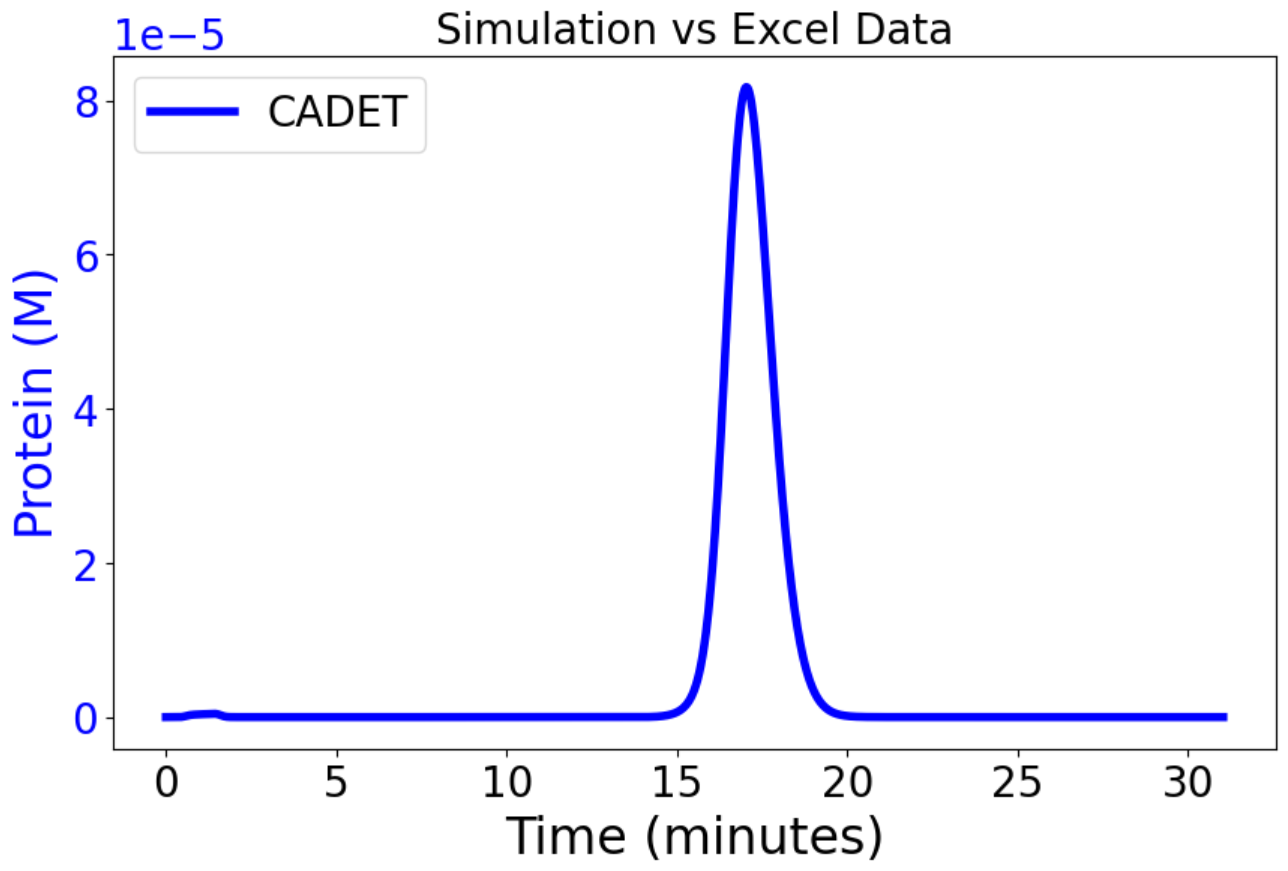
I can’t reproduce your plots exactly because they refer to a ‘hic_10_pro3.xlsx’ file that I don’t have, but here’s the CADET side. However, the timing is still a bit off compared to your plot.
Taking into account what @j.schmoelder said, I tried to convert the parameters that use the volume of the stationary phase from lumped stationary phase to solid stationary phase, just to see what happens. Assuming GoSilico runs in \frac{mol}{V_{stationary}} and CADET in \frac{mol}{V_{solid}} with V_{stationary} = V_{solid} + V_{pores} and V_{pores} = V_{stationary}*\varepsilon_p we have a ratio of \frac{1}{1-\varepsilon_p}\frac{V_{stationary}}{V_{solid}}
We can now convert between the two with: \frac{mol}{V_{stationary}} = \frac{mol}{V_{stationary}}*\frac{1}{1-\varepsilon_p}\frac{V_{stationary}}{V_{solid}} = \frac{1}{1-\varepsilon_p}\frac{mol}{V_{solid}}
i.e. by dividing concentrations by (1-\varepsilon_p). This now gives profiles that have all elutions at the correct time, but with too wide elution profiles:
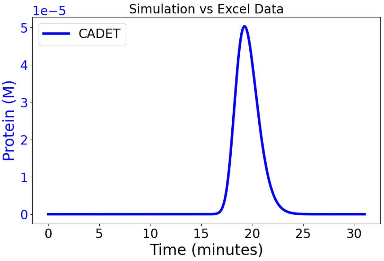
That GoSilico and CADET have different transport predictions is something we’ve seen before, but in the other direction, with CADET predicting too narrow of elutions.
Either way, as it is the weekend* and I’ve satiated my curiosity that the WHS isotherm can be approximately reproducible on both systems if the unit systems are considered, I’ll leave it at this.
*: (I’m not employed by the CADET Team anymore, so this is just me being curious in my free time)
Here’s the code for the plots in this post:
import os
import numpy as np
import pandas as pd
import matplotlib.pyplot as plt
import warnings
from CADETProcess.processModel import (
    Inlet, Outlet, LumpedRateModelWithPores,
    HICWaterOnHydrophobicSurfaces, ComponentSystem,
    FlowSheet, Process
)
from CADETProcess.simulator import Cadet
warnings.filterwarnings("ignore")

concentration_factor = 1/1000
ref_vol_factor = 1/(1 - 0.7571)

def run_single_simulation(flow_sheet, Vg, Vl, tag):
    simulator = Cadet()
    process = create_process(flow_sheet, Vg, Vl, tag)
    simulator.timeout = 6
    result = simulator.simulate(process)

    return tag, result, process
def create_process(flow_sheet, V_grad, V_load, tag):
    process = Process(flow_sheet, f"{tag}")
    wash_start = V_load / Q_m3_s
    grad_start = wash_start + 5e-6 / Q_m3_s
    grad_end = grad_start + V_grad / Q_m3_s
    sim_state[f"grad_end_{tag}"] = grad_end

    c_load = [starting_salt_conc, 0.136986*concentration_factor]
    c_wash = [starting_salt_conc, 0.0]
    c_elute = [75.2968*concentration_factor, 0.0]
    slope = (np.array(c_elute) - np.array(c_wash)) / (grad_end - grad_start)
    c_gradient_poly = list(zip(c_wash, slope))

    process.cycle_time = grad_end + 5e-6 / Q_m3_s
    process.add_event('load', 'flow_sheet.inlet.c', c_load)
    process.add_event('wash', 'flow_sheet.inlet.c', c_wash, wash_start)
    process.add_event('grad_start', 'flow_sheet.inlet.c', c_gradient_poly, grad_start)
    process.add_event('elute_start', 'flow_sheet.inlet.c', c_elute, grad_end)
    return process

component_system = ComponentSystem()
component_system.add_component('Salt')
component_system.add_component('Protein3')

binding = HICWaterOnHydrophobicSurfaces(component_system, name='HIC')
binding.is_kinetic = 1

equi = 3.89*ref_vol_factor
kinetic = 4.935
b0 = 0.0001048
b1 = 0.00450/concentration_factor
keff = 0.01e-3
n = 7.6
qmax = 48.7*concentration_factor*ref_vol_factor


Q_ml_min = 0.5
Q_m3_s = Q_ml_min / (60 * 1e6)
CV1 = 0.501437e-6
starting_salt_conc = 2083.45*concentration_factor
sim_state = {}

des_rate = 1 / kinetic
ads_rate = des_rate * equi

binding.adsorption_rate = [0.0, ads_rate]
binding.desorption_rate = [0.0, des_rate]
binding.hic_characteristic = [0.0, n]
binding.capacity = [0.0, qmax]
binding.beta_0 = b0
binding.beta_1 = b1
binding.bound_states = [0, 1]

inlet = Inlet(component_system, name='inlet')
inlet.flow_rate = Q_m3_s

column = LumpedRateModelWithPores(component_system, name='column')
column.binding_model = binding
column.length = 0.02
column.diameter = 0.00565
column.bed_porosity = 0.30
column.particle_radius = 4.5e-05
column.particle_porosity = 0.7571
column.axial_dispersion = 5.6e-8
column.film_diffusion = [0.01e-3, keff]
column.c = [starting_salt_conc, 0]
column.cp = [starting_salt_conc, 0]
column.q = [0]
column.discretization.ncol = 50

outlet = Outlet(component_system, name='outlet')


flow_sheet = FlowSheet(component_system)
flow_sheet.add_unit(inlet)
flow_sheet.add_unit(column)
flow_sheet.add_unit(outlet)
flow_sheet.add_connection(inlet, column)
flow_sheet.add_connection(column, outlet)

Vg, Vl, tag = 10 * CV1, 0.5e-6, 0

try:
    tag, result, process = run_single_simulation(flow_sheet, Vg, Vl, tag)
    sim_time = result.solution.outlet.outlet.time / 60  # Convert to minutes
    sim_concentration = result.solution.outlet.outlet.total_concentration_components[:, 1]
    sim_salt=result.solution.outlet.outlet.total_concentration_components[:, 0]
except Exception as e:
    print("Simulation failed:", e)

# excel_file_path = 'hic_10_pro3.xlsx'
# excel_data = pd.read_excel(excel_file_path)

# time_from_excel = excel_data['Time [min]']
# concentration_from_excel = excel_data['Biomolecule Concentration [mM]']


fig, ax1 = plt.subplots(figsize=(10, 6))

ax1.plot(sim_time, sim_concentration, label="CADET", color='b')
# ax1.plot(time_from_excel, concentration_from_excel, label="GoSilico", color='r', linestyle='--')

ax1.set_xlabel('Time (minutes)')
ax1.set_ylabel('Protein (M)', color='b')
ax1.tick_params(axis='y', labelcolor='b')

plt.title('Simulation vs Excel Data')
ax1.legend(loc='upper left')
plt.show()
To summarize:
- The WHS isotherm is sensitive to the unit system used. i.e. mol / L will give different results than mol / m^3 → we need to run CADET in mol / L to reproduce GoSilico results (which always runs in mol / L) approximately.
Additionally, differences in reference volumes are probably a confounding factor. As the isotherm is unit-system-dependent, the difference in reference volumes is something we will never be able to compensate without re-writing our model code.As per Shobhiths answer, the change in 1. was enough.- Similar results are possible with both systems, but exact matches depend on too many factors that we don’t know about.
- Without access to a GoSilico license and lots of time to systematically test parameters (of which I have neither), I can’t say more, but I hope this helps.