I have been able to set up a minimum reproducible example to replicate the issue in Rosario’s original post.
# -*- coding: utf-8 -*-
"""
This is a colloidal isotherm example for fitting lnKe and Bpp parameters
using U_NSGA3 with a callback and forward simulation.
1) User provides "true" parameters
2) A forward simulation is run using those parameters
3) The result of the forward simulation is used as a reference for optimization
4) The results of optimization are used for a forward simulation and plotted

The same functions are used to set up the optimization and forward simulation
"""
import matplotlib.pyplot as plt
from CADETProcess.processModel import ComponentSystem
from CADETProcess.processModel import MultiComponentColloidal
from CADETProcess.processModel import Inlet, Outlet, GeneralRateModel
from CADETProcess.processModel import FlowSheet, Process
from CADETProcess.simulator import Cadet
from CADETProcess.reference import ReferenceIO
from CADETProcess.comparison import Comparator
from CADETProcess.optimization import OptimizationProblem
from CADETProcess.optimization import U_NSGA3, Joblib


def set_binding_model(component_system, lnKe, Bpp):
    binding_model = MultiComponentColloidal(component_system, name='MultiComponentColloidal')
    binding_model.is_kinetic = True

    binding_model.phase_ratio = 1.46e8
    binding_model.kappa_exponential = 0
    binding_model.kappa_factor = 0
    binding_model.kappa_constant = 4e-9
    binding_model.coordination_number = 6

    binding_model.logkeq_exponent_factor = [0, lnKe]
    binding_model.logkeq_exponent_multiplier = [0, 0]
    binding_model.logkeq_power_exponent = [0, 0]
    binding_model.logkeq_power_factor = [0, 0]
    binding_model.logkeq_ph_exponent = [0, 0]

    binding_model.bpp_exponent_factor = [0, Bpp]
    binding_model.bpp_exponent_multiplier = [0, 0]
    binding_model.bpp_power_exponent = [0, 0]
    binding_model.bpp_power_factor = [0, 0]
    binding_model.bpp_ph_exponent = [0, 0]

    binding_model.protein_radius = [0, 4.5e-9]
    binding_model.kinetic_rate_constant = 1e8
    binding_model.bound_states = [0, 1]

    return binding_model


def set_column_model(component_system, binding_model):
    column = GeneralRateModel(component_system, name='column')

    column.discretization.ncol = 35
    column.discretization.npar = 35

    column.binding_model = binding_model

    column.length = 0.02
    column.diameter = 0.005
    column.cross_section_area = 1.96e-5
    column.particle_radius = 44e-6
    column.bed_porosity = 0.31
    column.particle_porosity = 0.90

    column.axial_dispersion = 2.85e-08
    column.film_diffusion = [9.86e-05, 1.14e-05]
    column.pore_diffusion = [6.5e-10, 3.71e-12]
    column.surface_diffusion = [0]

    column.c = [1e3*10**(-7.0), 0]
    column.cp = [1e3*10**(-7.0), 0]
    column.q = [0]

    return column


def make_process(lnKe, Bpp):
    component_system = ComponentSystem(['H+', 'protein'])

    binding_model = set_binding_model(component_system, lnKe, Bpp)
    column = set_column_model(component_system, binding_model)

    outlet = Outlet(component_system, name='outlet')

    load = Inlet(component_system, name='load')
    load.c = [1e3*10**(-7.0), 0.027]

    wash = Inlet(component_system, name='wash')
    wash.c = [1e3*10**(-7.0), 0]

    flow_sheet = FlowSheet(component_system)

    flow_sheet.add_unit(load)
    flow_sheet.add_unit(wash)
    flow_sheet.add_unit(column)
    flow_sheet.add_unit(outlet)

    flow_sheet.add_connection(load, column)
    flow_sheet.add_connection(wash, column)
    flow_sheet.add_connection(column, outlet)

    process = Process(flow_sheet, name='proc')
    process.cycle_time = 7920

    # set events
    process.add_event('load_on', 'flow_sheet.load.flow_rate', 3.68e-9, time=0)
    process.add_event('load_off', 'flow_sheet.load.flow_rate', 0, time=5520)
    process.add_event('wash_on', 'flow_sheet.wash.flow_rate', 3.68e-9, time=5520)
    process.add_event('wash_off', 'flow_sheet.wash.flow_rate', 0, time=7920)

    return process


def set_optimization_problem(time, data, process):
    def callback(simulation_results, individual, evaluation_object, callbacks_dir='./'):
        comparator = comparators[evaluation_object.name]
        comparator.plot_comparison(
            simulation_results,
            file_name=f'{callbacks_dir}/{individual.id}_{evaluation_object}_comparison.png',
            show=False
        )

    optimization_problem = OptimizationProblem('fit')

    simulator = Cadet()
    optimization_problem.add_evaluator(simulator)

    comparators = dict()

    optimization_problem.add_evaluation_object(process, name=process.name)

    fit_component_system = ComponentSystem(['protein'])
    reference = ReferenceIO(name=process.name, time=time, solution=data,
                            component_system=fit_component_system)

    comparator = Comparator(process.name)
    comparator.add_reference(reference)
    comparator.add_difference_metric('NRMSE', reference, 'outlet.inlet', components='protein')

    comparators[process.name] = comparator

    optimization_problem.add_objective(
        comparator,
        name=f"Objective {process.name}",
        evaluation_objects=[process],  # limit this comparator to be applied to only this one process
        n_objectives=comparator.n_metrics,
        requires=[simulator]
    )

    optimization_problem.add_variable(
        name='lnKe',
        parameter_path='flow_sheet.column.binding_model.logkeq_exponent_factor',
        indices=1,
        lb=5, ub=100,
        transform='auto'
    )

    optimization_problem.add_variable(
        name='Bpp',
        parameter_path='flow_sheet.column.binding_model.bpp_exponent_factor',
        indices=1,
        lb=1, ub=10,
        transform='auto'
    )

    optimization_problem.add_callback(callback, requires=[simulator])

    return optimization_problem


def run_fit(lnKe, Bpp):
    simulator = Cadet()

    # Create reference data with forward sim
    process = make_process(lnKe, Bpp)
    simulation_results = simulator.simulate(process)
    time = simulation_results.solution.outlet.outlet.time
    data = simulation_results.solution.outlet.outlet.solution
    data = data[:, 1].reshape(-1, 1)

    # Fit data from forward sim
    optimization_problem = set_optimization_problem(time, data, process)
    optimizer = U_NSGA3()
    optimizer.n_max_gen = 5
    optimizer.pop_size = 5
    # print(optimizer.options)

    # parallelize!!
    optimizer.backend = Joblib()
    optimizer.n_cores=-2

    print('\nCADET-Process optimization start!\n')
    optimization_results = optimizer.optimize(optimization_problem)
    print(f'Optimization completed in {optimization_results.time_elapsed:.2f} seconds.\n')

    # Create a new process from the fitting results
    fwd_process = make_process(optimization_results.x[0][0], Bpp)
    print(f'\nFitted lnKe: {optimization_results.x[0][0]:.2f}\n')
    print(f'\nFitted Bpp: {optimization_results.x[0][1]:.2f}\n')

    print('\nForward simulation start!\n')
    simulation_results = simulator.simulate(fwd_process)
    print(f'Simulation completed in {simulation_results.time_elapsed:.2f} seconds.\n')

    final_time = simulation_results.solution.outlet.outlet.time
    final_solution_array = simulation_results.solution.outlet.outlet.solution

    plt.plot(time, data, linestyle=':', color='k', label='reference')
    plt.plot(final_time, final_solution_array[:, 1], color='b', label='fit')
    plt.show()

    return optimization_results


if __name__=='__main__':
    run_fit(45, 4)
When running the code with the current values (lnKe=45, Bpp=4), the output I get is
CADET-Process optimization start!

==========================================================
n_gen  |  n_eval  | n_nds  |      eps      |   indicator
==========================================================
     1 |        5 |      1 |             - |             -
Finished Generation 1.
x: [72.88335145  8.99147563], f: [0.05533086]
     2 |       10 |      1 |  0.0348061575 |         ideal
Finished Generation 2.
x: [77.39609336  7.6842273 ], f: [0.0205247]
     3 |       15 |      1 |  0.0032067216 |         ideal
Finished Generation 3.
x: [75.48185755  7.68450607], f: [0.01731798]
     4 |       20 |      1 |  0.000000E+00 |             f
Finished Generation 4.
x: [75.48185755  7.68450607], f: [0.01731798]
     5 |       25 |      1 |  0.000000E+00 |             f
Finished Generation 5.
x: [75.48185755  7.68450607], f: [0.01731798]
Optimization completed in 264.72 seconds.

Fitted lnKe: 75.48
Fitted Bpp: 7.68

Forward simulation start!

Simulation completed in 23.27 seconds.
The parameter and objective values reported in the results_pareto.csv file that CADET_Process generates match those output in the terminal. The results of using these parameters in a forward simulation looks like this
which is expected because the parameters from the optimization are very different from the “true” values initially provided for the reference data.
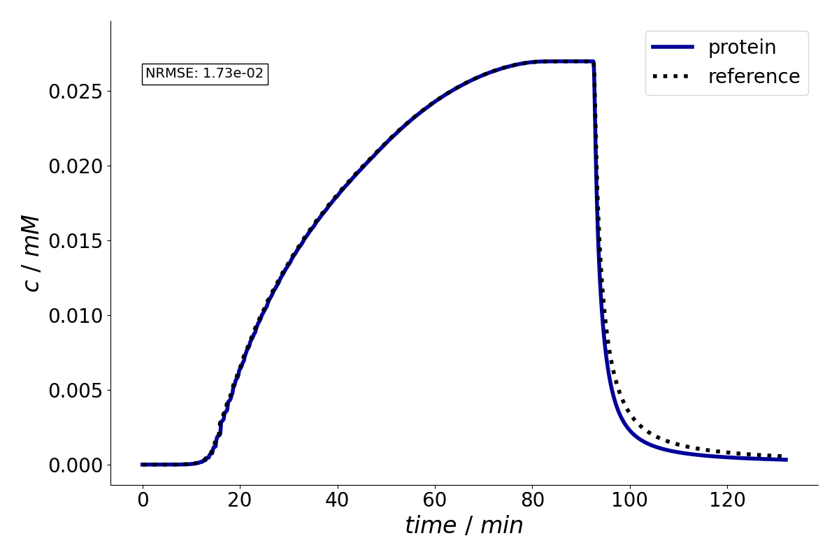
However, the CADET-Process callback plot looks like this:
The NRMSE matches the one from the terminal output and results_pareto.csv but the plot for the callback seems to be using different (and at least in this case better) parameters.
I haven’t figured out exactly when this difference happens and when it doesn’t, but I noticed that at least a few times when I was fitting only lnKe and not also fitting Bpp the two plots matched.
Previously, it had seemed like reducing the number of generations sometimes led to matching plots. Using the script above I have found that
optimizer.n_max_gen=1, optimizer.pop_size=5 → plot’s don’t match
optimizer.n_max_gen=1, optimizer.pop_size=1 → plot’s match
So it seems like maybe parameter sets are getting mixed up somewhere
Here’s my environment
environment.yml (13.1 KB)