Not understanding "is_kinetic" parameter

Ronan1234 · June 25, 2024, 9:20pm

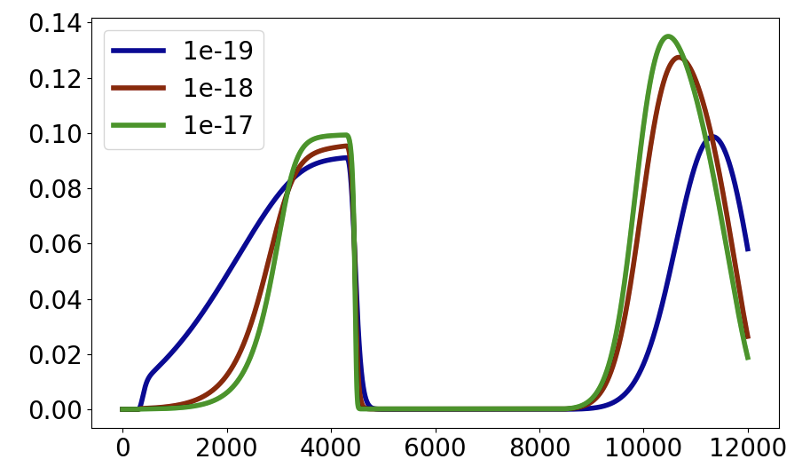
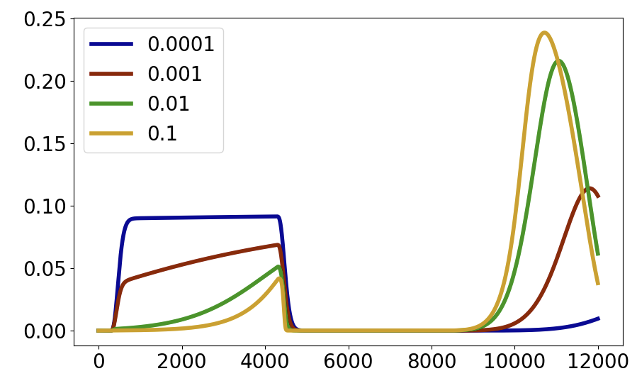
I do not understand the is_kinetic parameter. I got same results in CADET-Process for SMA binding using is_kinetic = True or False. Then, I tried reading Binding models — CADET and thought maybe it is only relevant for Langmuir and Langmuir LDF. But even then, the results for Langmuir with is_kinetic True is same as when is_kinetic is False.

In addition, the results for Langmuir LDF where I put driving_force_coefficient as 1 and appropriately adjust equilibrium_constant such that equilibrium_constant of LangmuirLDF is same as adorption/desorption of Langmuir, the results are again same and is_kinetic being True or False is not making any difference.

This is the code:

import numpy as np

from CADETProcess.processModel import ComponentSystem
from CADETProcess.processModel import Langmuir, LangmuirLDF
from CADETProcess.processModel import Inlet, GeneralRateModel, Outlet
from CADETProcess.processModel import FlowSheet
from CADETProcess.processModel import Process

component_system = ComponentSystem()
component_system.add_component('Protein 1')
component_system.add_component('Protein 2')

# binding_model = Langmuir(component_system, name='Lang')
# binding_model.is_kinetic = False
# binding_model.adsorption_rate = [1.3, 1.5]
# binding_model.desorption_rate = [0.5, 1.0]
# binding_model.capacity = 1
binding_model = LangmuirLDF(component_system, name='LangLDF')
binding_model.is_kinetic = True #False
binding_model.equilibrium_constant = [2.6, 1.5]
binding_model.driving_force_coefficient = [1.0, 1.0]
binding_model.capacity = 1

inlet = Inlet(component_system, name='inlet')
inlet.flow_rate = 2.88e-8

column = GeneralRateModel(component_system, name='column')
column.binding_model = binding_model

column.length = 0.65
column.diameter = 0.011286
column.bed_porosity = 0.37
column.particle_radius = 4.5e-5
column.particle_porosity = 0.33
column.axial_dispersion = 2.0e-7
column.film_diffusion = [2.0e-7, 2.0e-7]
column.pore_diffusion = [1e-7, 1e-7]
column.surface_diffusion = [0.0, 0.0]

outlet = Outlet(component_system, name='outlet')

# Flow Sheet
flow_sheet = FlowSheet(component_system)

flow_sheet.add_unit(inlet)
flow_sheet.add_unit(column)
flow_sheet.add_unit(outlet)

flow_sheet.add_connection(inlet, column)
flow_sheet.add_connection(column, outlet)

# Process
process = Process(flow_sheet, 'lwe')
process.cycle_time = 12000.0

## Create Events and Durations
wash_start = 400

_ = process.add_event('load', 'flow_sheet.inlet.c', [0.1, 0.1])
_ = process.add_event('wash', 'flow_sheet.inlet.c', [0.0, 0.0], wash_start)


column.c = [0, 0]
column.q = [0, 0]

ronald.jaepel · June 26, 2024, 10:03am

Hey Ronan,

you’ve set your system up in such a way, that the Langmuir binding reaches equilibrium so fast it’s in rapid equilibrium either way. Try a lower driving force, such as 0.01 or 0.001 . Here are two simulations with a driving force coefficient of 0.01 and is_kinetic True or False:

As explained in the documentation on the LDF versions:

All three approaches are equivalent in rapid equilibrium (IS_KINETIC = 0) but not equivalent when binding kinetics are considered (IS_KINETIC = 1).

So, to see differences between Langmuir and LangmuirLDF we need to use settings where the binding dynamics make a significant difference. Such as with a driving force coefficient of 0.01:

Or a driving force coefficient of 0.001

The same goes for the SMA isotherm. You need to use slow (i.e. low) values for ka and kd to create noticeable differences between kinetic and rapid equilibrium. Divide both by 10 as many times as necessary until you see a difference.

Ronan1234 · June 26, 2024, 2:54pm

Thanks for the response.
I was able to replicate this for Langmuir and LangmuirLDF however for SMA, even with very small ka = 3e-7and kd=1.5e-8 I get the same graph with or without is_kinetic (also tried very small kd of 1.5e-5 but higher ka of 3e-2)

import numpy as np

from CADETProcess.processModel import ComponentSystem
from CADETProcess.processModel import StericMassAction
from CADETProcess.processModel import Inlet, GeneralRateModel, Outlet
from CADETProcess.processModel import FlowSheet
from CADETProcess.processModel import Process

component_system = ComponentSystem()
component_system.add_component('Salt')
component_system.add_component('Protein 1')
component_system.add_component('Protein 2')

binding_model = StericMassAction(component_system, name='SMA')
binding_model.is_kinetic = True #False #
binding_model.adsorption_rate = [0, 3e-7, 3e-7] #[0.0, 3, 3]
binding_model.desorption_rate = [0, 1.5e-8, 1.5e-8] #[0.0, 15, 15]
binding_model.characteristic_charge = [0.0, 7.0, 7.0]
binding_model.steric_factor = [0.0, 50.0, 50.0]
binding_model.capacity = 225.0

inlet = Inlet(component_system, name='inlet')
inlet.flow_rate = 2.88e-8

column = GeneralRateModel(component_system, name='column')
column.binding_model = binding_model

column.length = 0.25
column.diameter = 0.011286
column.bed_porosity = 0.37
column.particle_radius = 4.5e-5
column.particle_porosity = 0.33
column.axial_dispersion = 2.0e-7
column.film_diffusion = [2.0e-5, 2.0e-7, 2.0e-7]
column.pore_diffusion = [7e-5, 1e-9, 1e-9]
column.surface_diffusion = [0.0, 0.0, 0.0]

outlet = Outlet(component_system, name='outlet')

# Flow Sheet
flow_sheet = FlowSheet(component_system)

flow_sheet.add_unit(inlet)
flow_sheet.add_unit(column)
flow_sheet.add_unit(outlet)

flow_sheet.add_connection(inlet, column)
flow_sheet.add_connection(column, outlet)

# Process
process = Process(flow_sheet, 'lwe')
process.cycle_time = 12000.0

## Create Events and Durations
wash_start = 4000 #4000.0
gradient_start = 8000 #8000.0
concentration_difference = np.array([500.0, 0.0]) - np.array([180.0, 0.0])
gradient_duration = process.cycle_time - gradient_start
gradient_slope = concentration_difference/gradient_duration

_ = process.add_event('load', 'flow_sheet.inlet.c', [180.0, 0.1, 0.1])
_ = process.add_event('wash', 'flow_sheet.inlet.c', [70.0, 0.0, 0.0], wash_start)
_ = process.add_event(
    'grad_start',
    'flow_sheet.inlet.c',
    [[70.0, gradient_slope[0]], [0, gradient_slope[1]], [0, gradient_slope[1]]],
    gradient_start
)

column.c = [180, 0, 0]
column.q = [binding_model.capacity, 0, 0]

ronald.jaepel · June 26, 2024, 7:39pm

For the SMA without reference concentrations, ka and kd go to absurdly high or low values.
To see kinetic effects we need to lower ka was far as 1e-19 to 1e-17 (while lowering kd along with it to keep Keq constant)

If we use reference concentrations (and set both to 225)

    binding_model.reference_solid_phase_conc = 225.0
    binding_model.reference_liquid_phase_conc = 225.0

this brings the range of Ka values where kinetic effects are visible to 0.1 - 1e-4.

We generally recommend the use of reference concentrations. Be aware that you’ll need to transform your Ka and kd to get identical simulations. How to do that is described in the documentation I linked above.