Hi everyone,
I’ve been setting up the 6-component IEX case study from Meyer et al., 2026, ChromOps.jl (Section 4.2) as I thought it’d be a good standard benchmark for the CADET testing pipelines.
To this end, I mapped the paper's equations onto CADET's
The paper’s q_i is per pore-liquid volume, while CADET’s c^s_i is per solid volume. With
CADET’s pore balance
becomes the paper’s Eq. (2) exactly for k^f_i = \varepsilon^p r^p k_{\mathrm{MT},i}/3, and the same k^f_i turns CADET’s bulk film term \frac{1-\varepsilon^b}{\varepsilon^b}\frac{3}{r^p}k^f_i into the paper’s \frac{(1-\varepsilon^b)\varepsilon^p}{\varepsilon^b}k_{\mathrm{MT},i}. Since only the ratio k^f_i/r^p enters CADET, r^p can be chosen freely as long as CADET’s k^f is computed from it.
CADET’s SMA at equilibrium, solved for c^p_i:
Now substitute \Lambda^{C}=\Lambda/\alpha and c^s_j=q_j/\alpha, which pulls a common 1/\alpha out of the denominator:
Together with c^s_i=q_i/\alpha, the two powers of α collect into \alpha^{\nu_i-1}:
the paper’s Eq. (4) at equilibrium. The underbrace is where k^a_i/k^d_i=k^{eq}_i\alpha^{\nu_i-1} is used.
CADET’s c^s_0=\Lambda^{C}-\sum_j\nu_j c^s_j, multiplied by \alpha, gives q_0=\Lambda-\sum_j\nu_j q_j, which is Eq. (5) from the paper. The initial condition has to carry the factor too: INIT_CS[0] =\Lambda/\alpha = 630.3 mol/m³, which is the paper’s q_s(0)=\Lambda=324.7 mol/m³.
However, I can’t reproduce Figure 1 from the reported equations and parameters, and I’d like to check whether I’ve misread something.
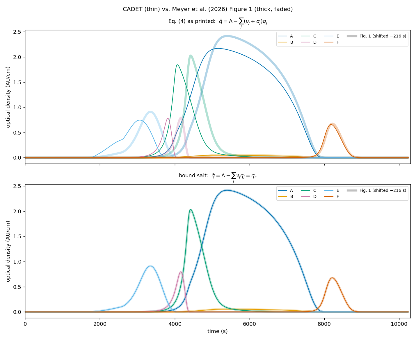
There seem to be two separate issues:
- The salt outlet delay should be fixed by Table 3 alone: (\varepsilon^b + (1−\varepsilon^b) \varepsilon^p) \cdot L/(\varepsilon^b v_{int}) = 283 s, independent of k_MT and D_ax. My simulation reproduces that but Figure 1 from the paper shows a delay of ~499 s.
- Peak heights/shape and spacing: With the SMA Eq. (4) from the paper, the six peaks come out up to 18% low and with different shape. If I instead use the bound-salt concentration q_s = \Lambda - \sum_j \nu_j q_j in the denominator of Eq. 4 (achieved by setting the shielding factor \sigma_i = 0\ \forall i), every peak height is reproduced to within 0.5 % and the peak shape is right: normalized RMSE drops from 20 % to 0.18 % (after applying the offset descibed in point 1). However, the paper explicitly reports \sigma_i = 3 which is why I suspect I’m overlooking something rather than that the equation is wrong.
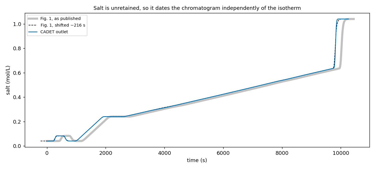
My python script for the CADET simulation reported above is here: https://github.com/cadet/CADET-Verification/pull/163
Maybe the author @krismey can help me out? 
Thanks in advance!