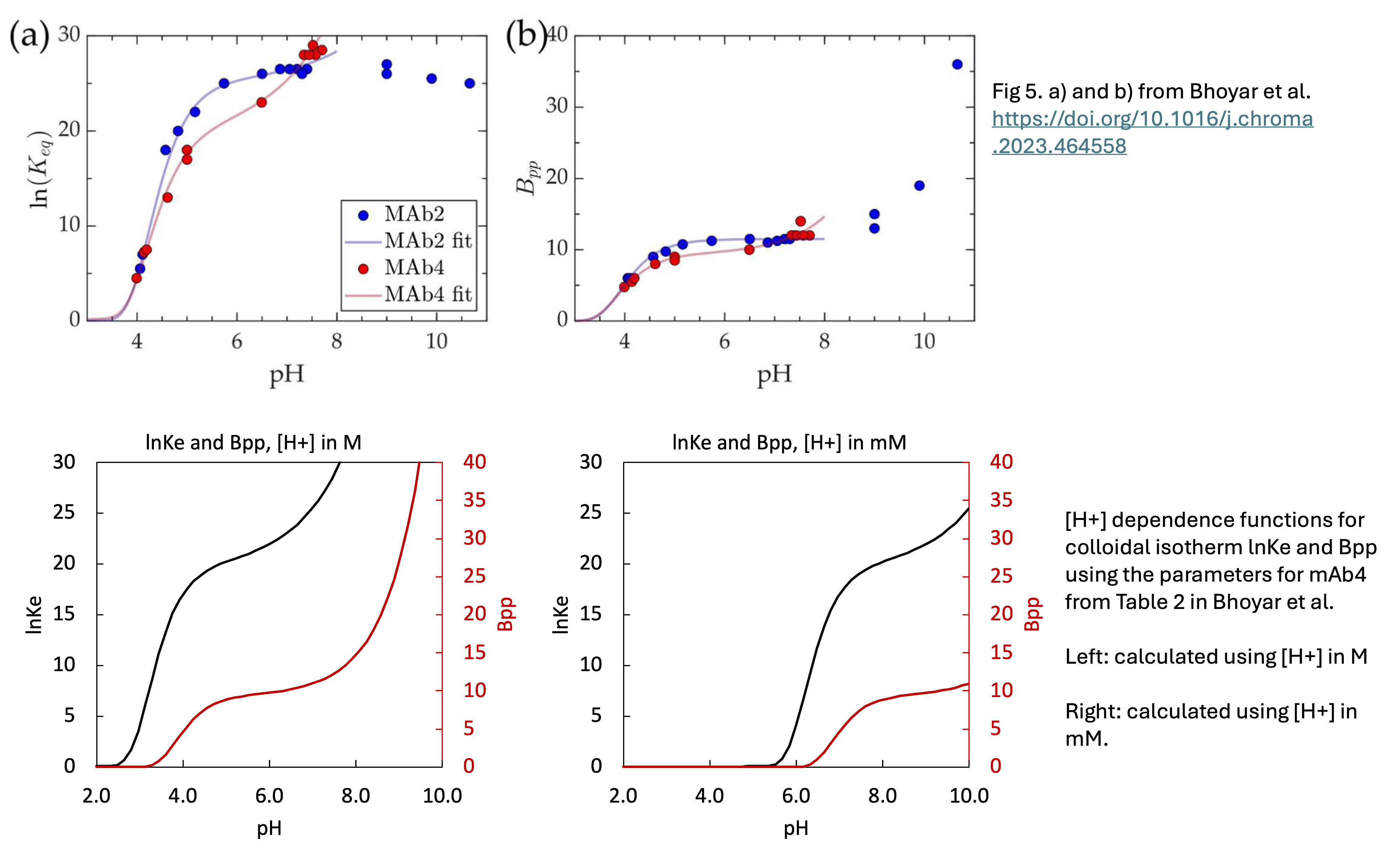
Hello community,
I am new to CADET modeling and still gaining familiarity with chromatography process modeling. I am currently working on reproducing the simulated chromatograms presented in: “Bhoyar, S.; Kumar, V.; Foster, M.; Xu, X.; Traylor, S.; Guo, J.; Lenhoff, A.: Predictive mechanistic modeling of loading and elution in protein A chromatography, Journal of Chromatography A 1713 (2024): 464558” Specifically, I am attempting to replicate the chromatograms shown in Figures 10a, 10b, and 10c (Section 3.2.2) using CADET-Python. I implemented the reported model architecture, unit operations, solver settings, and isotherm parameters as described in the article. However, I had to make two assumptions due to missing details:
-
pH Inlet Profile Construction:
I manually parameterized the inlet pH trajectory based on Section 2.2.3 of the paper, i.e., constant pH 7.5 during load and wash, followed by a linear gradient to pH 3.5 over 25 CV for elution. -
Loading Duration Estimation:
As the manuscript does not explicitly state the loading duration for the simulations, I inferred these values from the experimental chromatograms shown (e.g., ~115 CV for Figure 10b).
While my simulated loading curves show small differences compared to the paper, the deviations during the wash and particularly elution steps are more pronounced.
Key discrepancies include:
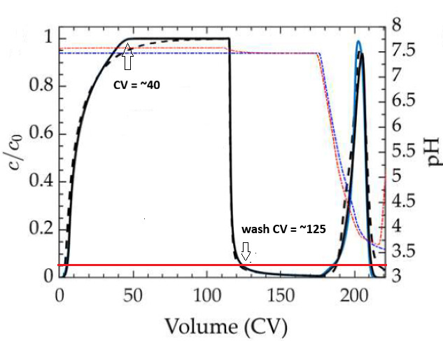
a) Significant loss of mAb during the wash phase, which is not observed in the published simulations
b) Earlier onset of elution
c) Lower elution peak height
d) Outlet pH at peak maximum deviates from the published curves
e) Overall chromatogram shape differs from the solid black simulation curves in the paper
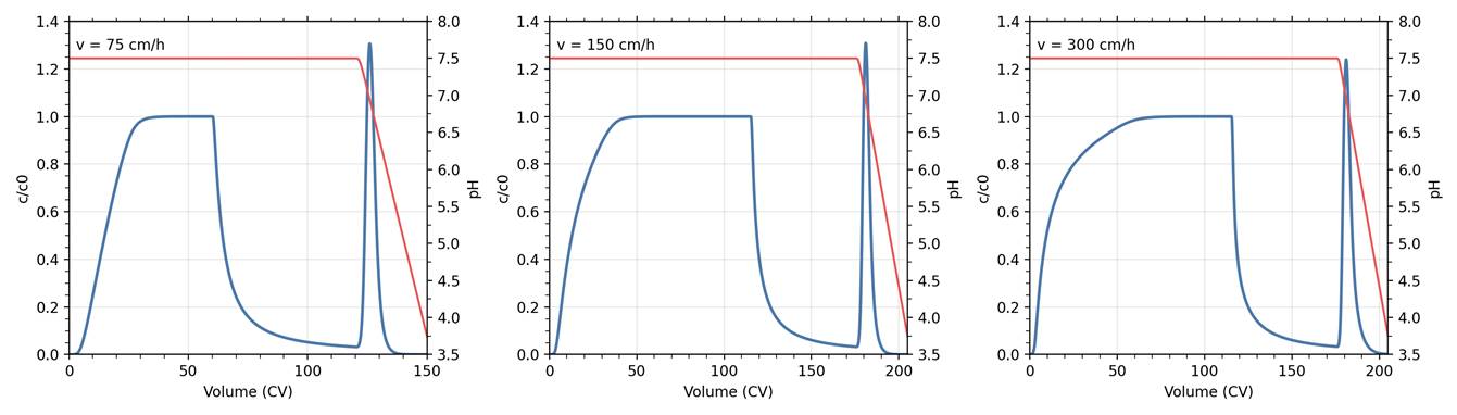
For reference, I have attached representative plots (blue = chromatogram, red = outlet pH) below. I have also included my full CADET-Python script at the end of this post.
-
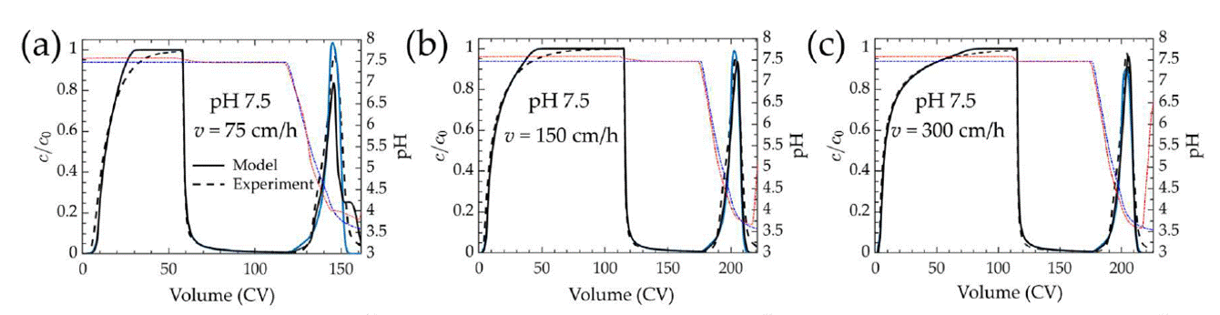
from the article (fig 10 a–c)
-
from my code
Given the differences described above, I would greatly appreciate insight from the community. Any suggestions, corrections, or perspectives would be extremely valuable.
Thank you in advance for your time and help.
Code:
#!/usr/bin/env python3
"""
Standalone reproduction script for a 1x3 chromatogram panel (L=2.5 cm, c0=6 mg/mL)
with outlet pH on a secondary y-axis and top x-axis ticks (no labels).
Runs CADET if H5 files are missing.
"""
import os
import math
import numpy as np
import h5py
try:
from cadet import Cadet
except Exception as exc:
raise RuntimeError("cadet-python is required to run this script") from exc
OUTPUT_DIR = os.path.join(os.path.dirname(__file__), "out")
OUTPUT_PNG = os.path.join(OUTPUT_DIR, "chromatograms_L2.5_c6_v75_v150_v300_panel_repro.png")
# Column and system
ID = 0.03
R = ID / 2.0
EPS_C = 0.40
EPS_P = 0.65
R_P = 44e-6
LENGTH_CM = 2.5
# Transport
D_AX = 1.0e-6
K_FILM = 1.0e-5
D_P = 4.0e-12
D_H = 1e-9
# Colloidal constants
A_PROT = 4.5e-9
PHI = 1.6e8
KAPPA_MAB4 = 5.3e-9
# Discretization
NCOL = 60
NPAR = 45
ABS_TOL = 1e-8
REL_TOL = 1e-6
N_TIME_POINTS = 2000
SENSITIVITY_TIME_POINTS = 500
MW_MAB = 150000.0
SURF_DIFF_Hp = 0.0
SURF_DIFF_PROTEIN = 4.6e-14
SURF_DIFF_DEP = "LIQUID_SALT_EXPONENTIAL"
SURF_DIFF_EXP_FACTOR_PROTEIN = 1.0
SURF_DIFF_EXP_ARGMULT_PROTEIN = -26800.0
PH_LOAD = 7.5
PH_END = 3.5
N_ELUT_SEGMENTS = 80
LOAD_CV_DEFAULT = 115.0
LOAD_CV_75 = 60.0
WASH_CV = 60.0
ELUT_CV = 30.0
VELOCITIES_CM_PER_H = [75.0, 150.0, 300.0]
C0_MG_ML = 6.0
RUN_SENSITIVITY = True
SENSITIVITY_REQUIRE_EXISTING = False
def mg_per_mL_to_mol_per_m3(c_mg_per_mL: float, mw_g_per_mol: float) -> float:
c_g_per_L = c_mg_per_mL
c_mol_per_L = c_g_per_L / mw_g_per_mol
return c_mol_per_L * 1000.0
def cv_to_time_s(cv_value: float, length_cm: float, velocity_cm_per_h: float) -> float:
u_s = (velocity_cm_per_h / 100.0) / 3600.0
t_per_CV = (length_cm / 100.0) / u_s if u_s else None
return float(cv_value) * t_per_CV if t_per_CV else None
def build_and_run(
length_cm,
velocity_cm_per_h,
c0_mg_ml,
h5_name,
transport_overrides=None,
n_time_points=None,
):
load_cv = LOAD_CV_75 if abs(velocity_cm_per_h - 75.0) < 1e-9 else LOAD_CV_DEFAULT
t_load = cv_to_time_s(load_cv, length_cm, velocity_cm_per_h)
t_wash = cv_to_time_s(WASH_CV, length_cm, velocity_cm_per_h)
t_elut = cv_to_time_s(ELUT_CV, length_cm, velocity_cm_per_h)
t_total = t_load + t_wash + t_elut
c0 = mg_per_mL_to_mol_per_m3(c0_mg_ml, MW_MAB)
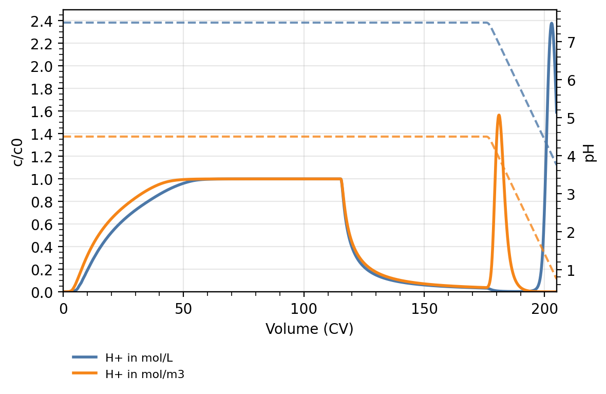
H_load = 10.0 ** (-PH_LOAD) * 1000.0
m = Cadet()
m.filename = os.path.abspath(os.path.join(OUTPUT_DIR, h5_name))
os.makedirs(os.path.dirname(m.filename), exist_ok=True)
ncomp = 2
m.root.input.model.nunits = 3
m.root.input.model.unit_000.unit_type = "INLET"
m.root.input.model.unit_000.ncomp = ncomp
m.root.input.model.unit_000.inlet_type = "PIECEWISE_CUBIC_POLY"
elut_dt = t_elut / N_ELUT_SEGMENTS if N_ELUT_SEGMENTS > 0 else t_elut
section_times = [0.0, t_load, t_load + t_wash]
for i in range(N_ELUT_SEGMENTS):
section_times.append(t_load + t_wash + (i + 1) * elut_dt)
m.root.input.solver.sections.nsec = len(section_times) - 1
m.root.input.solver.sections.section_times = section_times
m.root.input.solver.sections.section_continuity = [0] * (len(section_times) - 2)
m.root.input.model.unit_000.sec_000.const_coeff = [H_load, c0]
m.root.input.model.unit_000.sec_000.lin_coeff = [0.0, 0.0]
m.root.input.model.unit_000.sec_000.quad_coeff = [0.0, 0.0]
m.root.input.model.unit_000.sec_000.cube_coeff = [0.0, 0.0]
m.root.input.model.unit_000.sec_001.const_coeff = [H_load, 0.0]
m.root.input.model.unit_000.sec_001.lin_coeff = [0.0, 0.0]
m.root.input.model.unit_000.sec_001.quad_coeff = [0.0, 0.0]
m.root.input.model.unit_000.sec_001.cube_coeff = [0.0, 0.0]
# We approximate the H+ profile for elution section by splitting elution into many
# small segments, because H+ concentration is defined in terms of inlet pH: linear pH
# becomes a nonlinear H+ profile. Piecewise segments approximate the intended H+ profile.
for i in range(N_ELUT_SEGMENTS):
seg_start = t_load + t_wash + i * elut_dt
seg_end = seg_start + elut_dt
frac0 = (seg_start - (t_load + t_wash)) / t_elut if t_elut > 0 else 0.0
frac1 = (seg_end - (t_load + t_wash)) / t_elut if t_elut > 0 else 1.0
frac0 = min(max(frac0, 0.0), 1.0)
frac1 = min(max(frac1, 0.0), 1.0)
pH0 = PH_LOAD + (PH_END - PH_LOAD) * frac0
pH1 = PH_LOAD + (PH_END - PH_LOAD) * frac1
H0 = 10.0 ** (-pH0) * 1000.0
H1 = 10.0 ** (-pH1) * 1000.0
slope = (H1 - H0) / elut_dt if elut_dt > 0 else 0.0
sec_idx = 2 + i
sec = getattr(m.root.input.model.unit_000, f"sec_{sec_idx:03d}")
sec.const_coeff = [H0, 0.0]
sec.lin_coeff = [slope, 0.0]
sec.quad_coeff = [0.0, 0.0]
sec.cube_coeff = [0.0, 0.0]
col = m.root.input.model.unit_001
col.unit_type = "GENERAL_RATE_MODEL"
col.ncomp = ncomp
col.col_length = length_cm / 100.0
col.col_radius = R
col.col_porosity = EPS_C
col.par_porosity = EPS_P
col.par_radius = R_P
col.col_dispersion = D_AX
col.velocity = (velocity_cm_per_h / 100.0) / 3600.0
col.film_diffusion = [K_FILM, K_FILM]
col.par_diffusion = [D_H, D_P]
col.PAR_SURFDIFFUSION = [SURF_DIFF_Hp, SURF_DIFF_PROTEIN]
col.PAR_SURFDIFFUSION_DEP = SURF_DIFF_DEP
if SURF_DIFF_DEP == "LIQUID_SALT_EXPONENTIAL":
col.PAR_SURFDIFFUSION_EXPFACTOR = [0.0, SURF_DIFF_EXP_FACTOR_PROTEIN]
col.PAR_SURFDIFFUSION_EXPARGMULT = [0.0, SURF_DIFF_EXP_ARGMULT_PROTEIN]
col.discretization.ncol = NCOL
col.discretization.npar = NPAR
col.discretization.par_disc_type = "EQUIDISTANT"
col.discretization.use_analytic_jacobian = 1
col.discretization.use_implicit_volume = 1
col.discretization.gs_type = 1
col.discretization.max_krylov = 0
col.discretization.max_restarts = 10
col.discretization.schur_safety = 1e-8
col.discretization.use_weno = 0
col.discretization.weno.boundary_model = 0
col.discretization.weno.weno_eps = 1e-6
col.discretization.weno.weno_order = 3
col.adsorption_model = "MULTI_COMPONENT_COLLOIDAL"
col.adsorption.COL_PHI = PHI
col.adsorption.COL_CORDNUM = 6
col.adsorption.IS_KINETIC = 1
col.adsorption.COL_PROTEIN_RADIUS = [0, A_PROT]
col.adsorption.COL_USE_PH = 0
col.adsorption.COL_LINEAR_THRESHOLD = 1e-8
col.adsorption.COL_LOGKEQ_SALT_POWEXP = [0, 0.0133]
col.adsorption.COL_LOGKEQ_SALT_POWFACT = [0, 0.38]
col.adsorption.COL_LOGKEQ_SALT_EXPFACT = [0, 19.47]
col.adsorption.COL_LOGKEQ_SALT_EXPARGMULT = [0, -16000.0]
col.adsorption.COL_LOGKEQ_PH_EXP = [0, 0]
col.adsorption.COL_BPP_SALT_POWFACT = [0, 0.0004]
col.adsorption.COL_BPP_SALT_POWEXP = [0, -0.516]
col.adsorption.COL_BPP_SALT_EXPFACT = [0, 9.348]
col.adsorption.COL_BPP_SALT_EXPARGMULT = [0, -6993.0]
col.adsorption.COL_BPP_PH_EXP = [0, 0]
col.adsorption.COL_KKIN = [1e9, 1e9]
col.adsorption.COL_KAPPA_EXP = 0
col.adsorption.COL_KAPPA_FACT = 0
col.adsorption.COL_KAPPA_CONST = 1 / KAPPA_MAB4
if transport_overrides:
for key, value in transport_overrides.items():
setattr(col, key, value)
col.nbound = [0, 1]
col.init_c = [H_load, 0.0]
col.init_q = [0.0, 0.0]
m.root.input.model.unit_002.unit_type = "OUTLET"
m.root.input.model.unit_002.ncomp = ncomp
Q = col.velocity * math.pi * R * R
m.root.input.model.connections.nconn = 2
m.root.input.model.connections.nswitches = 1
m.root.input.model.connections.switch_000.section = 0
m.root.input.model.connections.switch_000.connections = [0, 1, -1, -1, Q, 1, 2, -1, -1, Q]
rgrp = m.root.input["return"]
rgrp.WRITE_SOLUTION_TIMES = 1
rgrp.SPLIT_COMPONENTS_DATA = 1
rgrp.SPLIT_PORTS_DATA = 1
rgrp.unit_001.WRITE_SOLUTION_OUTLET = 1
rgrp.unit_002.WRITE_SOLUTION_OUTLET = 1
m.root.input.solver.time_integrator.abstol = ABS_TOL
m.root.input.solver.time_integrator.reltol = REL_TOL
m.root.input.solver.time_integrator.algtol = 1e-10
m.root.input.solver.time_integrator.init_step_size = 1e-6
m.root.input.solver.time_integrator.max_steps = 1000000
m.root.input.model.solver.schur_safety = 1e-8
m.root.input.model.solver.gs_type = 1
m.root.input.model.solver.max_krylov = 0
m.root.input.model.solver.max_restarts = 10
time_points = N_TIME_POINTS if n_time_points is None else n_time_points
if time_points and t_total > 0:
m.root.input.solver.user_solution_times = np.linspace(0.0, t_total, time_points)
m.save()
ret = m.run_simulation()
if getattr(ret, "return_code", 1) not in (0, 1):
stderr = getattr(ret, "stderr", None)
stdout = getattr(ret, "stdout", None)
msg = f"CADET run failed (code={getattr(ret, 'return_code', None)})"
if stderr:
msg += f"\nSTDERR:\n{stderr}"
if stdout:
msg += f"\nSTDOUT:\n{stdout}"
raise RuntimeError(msg)
return m.filename
def read_outlet_comp(h5_path: str, comp_idx: int):
with h5py.File(h5_path, "r") as fh:
sol = fh.get("/output/solution") or fh.get("output/solution")
if sol is None:
return None, None
times = sol.get("SOLUTION_TIMES")[()]
unit = sol.get("unit_002") or sol.get("unit_001")
if unit is None:
return None, None
key = f"SOLUTION_OUTLET_COMP_{comp_idx:03d}"
if key in unit:
comp = unit[key][()]
else:
comp = None
for k in unit:
if "SOLUTION_OUTLET" in k.upper():
d = unit[k][()]
comp = d[:, comp_idx] if d.ndim == 2 else d
break
return times, comp
def main():
import matplotlib
matplotlib.use("Agg")
import matplotlib.pyplot as plt
os.makedirs(OUTPUT_DIR, exist_ok=True)
fig, axes = plt.subplots(1, 3, figsize=(14, 4), sharey=False)
for ax, v_cm_per_h in zip(axes, VELOCITIES_CM_PER_H):
h5_name = f"L{LENGTH_CM:.1f}_u{v_cm_per_h:.0f}_c{C0_MG_ML:.1f}.h5"
h5_path = os.path.join(OUTPUT_DIR, h5_name)
if not os.path.exists(h5_path):
h5_path = build_and_run(LENGTH_CM, v_cm_per_h, C0_MG_ML, h5_name)
times, comp1 = read_outlet_comp(h5_path, 1)
_, comp0 = read_outlet_comp(h5_path, 0)
if times is None or comp1 is None or comp0 is None:
if os.path.exists(h5_path):
os.remove(h5_path)
h5_path = build_and_run(LENGTH_CM, v_cm_per_h, C0_MG_ML, h5_name)
times, comp1 = read_outlet_comp(h5_path, 1)
_, comp0 = read_outlet_comp(h5_path, 0)
if times is None or comp1 is None or comp0 is None:
raise RuntimeError(f"Missing outlet data in {h5_path}")
u_s = (v_cm_per_h / 100.0) / 3600.0
t_per_CV = (LENGTH_CM / 100.0) / u_s
CV = times / t_per_CV
c0 = mg_per_mL_to_mol_per_m3(C0_MG_ML, MW_MAB)
c_over_c0 = comp1 / c0
ax.plot(CV, c_over_c0, color="#4C78A8", lw=2)
ax.set_xlabel("Volume (CV)")
ax.set_ylabel("c/c0")
x_max = float(np.nanmax(CV)) if np.size(CV) else 0.0
ax.set_xlim(0, x_max)
y_max = max(1.0, np.nanmax(c_over_c0) * 1.05)
y_max = math.ceil(y_max / 0.2) * 0.2
ax.set_ylim(0, y_max)
ax.text(0.02, 0.95, f"v = {v_cm_per_h:.0f} cm/h", transform=ax.transAxes, va="top", ha="left")
ax.set_xticks(np.arange(0, x_max + 1e-6, 50))
ax.set_xticks(np.arange(0, x_max + 1e-6, 10), minor=True)
ax.set_yticks(np.arange(0, y_max + 1e-9, 0.2))
ax.set_yticks(np.arange(0, y_max + 1e-9, 0.05), minor=True)
ax.tick_params(axis="x", which="minor", length=3)
ax.tick_params(axis="y", which="minor", length=3)
ax.grid(True, which="major", alpha=0.3)
outlet_pH = np.array([(-math.log10(v / 1000.0) if v > 0 else np.nan) for v in comp0])
ax2 = ax.twinx()
ax2.plot(CV, outlet_pH, color="#E45756", lw=1.5)
ax2.set_ylabel("pH")
pH_min = float(np.nanmin(outlet_pH)) if np.size(outlet_pH) else 0.0
pH_max = float(np.nanmax(outlet_pH)) if np.size(outlet_pH) else 1.0
if pH_max <= pH_min:
pH_min, pH_max = 0.0, 1.0
pH_min_tick = math.floor(pH_min * 2.0) / 2.0
pH_max_tick = math.ceil(pH_max * 2.0) / 2.0
ax2.set_yticks(np.arange(pH_min_tick, pH_max_tick + 1e-9, 0.5))
ax2.set_yticks(np.arange(pH_min_tick, pH_max_tick + 1e-9, 0.25), minor=True)
ax2.tick_params(axis="y", which="minor", length=3)
ax_top = ax.secondary_xaxis("top")
ax_top.set_xticks(np.arange(0, x_max + 1e-6, 50))
ax_top.set_xticks(np.arange(0, x_max + 1e-6, 10), minor=True)
ax_top.set_xlabel("")
ax_top.tick_params(axis="x", which="major", labeltop=False)
fig.tight_layout()
fig.savefig(OUTPUT_PNG, dpi=200)
plt.close(fig)
print(f"[INFO] Saved panel: {OUTPUT_PNG}")
if __name__ == "__main__":
main()