WENO for axisymmetric cylindrical settings

Hi there,

I’m working on implementing radial flow chromatography models. To this end, I’ve derived the interstitial volume equations as follows:

We start with the equation in coordinate-free form:

\frac{\partial c}{\partial t} = -\operatorname{div}( \vec{u} c) + \operatorname{div}(D_{\mathrm{rad}} \nabla c) + \frac{1- \varepsilon_c}{\varepsilon_c} \frac{3 k_f}{R_p} \left( \left.c^{(p)}\right|_{\rho=R_p} - c\right).

First, we focus on the convective term:

\operatorname{div}( \vec{u} c),

where \vec{u} is the velocity field und c is the concentration. Since the fluid is incompressible, we require

\operatorname{div}(\vec{u}) = 0.

Using cylindrical coordinates, assuming symmetry (i.e., c and \vec{u} only depend on radial position r), and using a strictly radial flow (i.e., \vec{u} = u \vec{e}_r, where \vec{e}_r is the unit vector in radial direction), this yields

\begin{aligned} 0 &= \operatorname{div}(\vec{u}) = \frac{1}{r} \frac{\partial}{\partial r}\left( r \vec{u} \cdot \vec{e}_r\right) + \frac{1}{r} \frac{\partial}{\partial \varphi}\left( \vec{u} \cdot \vec{e}_{\varphi}\right) + \frac{\partial}{\partial z}\left( \vec{u} \cdot \vec{e}_z\right) \\ &= \frac{1}{r} \frac{\partial}{\partial r}\left( r u \right) = \frac{u}{r} + \frac{\partial u}{\partial r}. \end{aligned}

The solution to this differential equation is

u(r) = \frac{v}{r},

where v \in \mathbb{R} is some constant. Concluding, for a divergence free velocity field with purely radial direction we need

\vec{u} = \frac{v}{r} \vec{e}_r.

Plugging this into the divergence term for the convection and applying cylindrical coordinates, we obtain

\operatorname{div}( \vec{u} c) = \operatorname{div}\left( c \frac{v}{r} \vec{e}_r\right) = \frac{1}{r} \frac{\partial}{\partial r}\left( r c \frac{v}{r} \right) = \frac{v}{r} \frac{\partial c}{\partial r}.

Second, the dispersive term is simply translated to cylindrical coordinates:

\operatorname{div}(D_{\mathrm{rad}} \nabla c) = D_{\mathrm{rad}} \frac{1}{r} \frac{\partial}{\partial r} \left( r \frac{\partial c}{\partial r} \right).

We finally arrive at

\frac{\partial c}{\partial t} = - \frac{v}{r} \frac{\partial c}{\partial r} + D_{\mathrm{rad}} \frac{1}{r} \frac{\partial}{\partial r} \left( r \frac{\partial c}{\partial r} \right) + \frac{1- \varepsilon_c}{\varepsilon_c} \frac{3 k_f}{R_p} \left( \left.c^{(p)}\right|_{\rho=R_p} - c\right).
3 Likes

When applying finite volumes (a FV cell is a cylindrical shell), we need to apply volume averages:

\frac{1}{V_i} \int_{V_i} f(x) \,\mathrm{d}x,

where the volume is given by V_i = \pi (r_{i+1}^2 - r_i^2) L. Here, L denotes the length of the column in axial direction. Let’s assume that f only depends on the radial position r. This yields

\begin{aligned} \frac{1}{V_i} \int_{V_i} f(x) \,\mathrm{d}x &= \frac{1}{\pi (r_{i+1}^2 - r_i^2) L} \int_{0}^L \int_0^{2\pi} \int_{r_i}^{r_{i+1}} f(r) r \,\mathrm{d}r \, \mathrm{d}\varphi \, \mathrm{d}z \\ &= \frac{2\pi L}{\pi (r_{i+1}^2 - r_i^2) L} \int_{r_i}^{r_{i+1}} f(r) r \,\mathrm{d}r \\ &= \frac{1}{r_{i+1/2} h_r} \int_{r_i}^{r_{i+1}} f(r) r \,\mathrm{d}r, \end{aligned}

where h_r = r_{i+1}-r_i is the (uniform) radial size of the shells and r_{i+1/2} = (r_{i+1} + r_i) / 2 is the radial midpoint of cell V_i.

Taking volume averages of the convective term, we yield

\frac{1}{r_{i+1/2} h_r} \int_{r_i}^{r_{i+1}} \frac{v}{r} \frac{\partial c}{\partial r} r \,\mathrm{d}r = \frac{v}{r_{i+1/2} h_r} \left[ c \right]_{r_i}^{r_{i+1}}.

Thus, we need to evaluate c at the radial cell edges r_{i+1} and r_i. Here, we want to apply a WENO scheme.

However, we cannot simply use the standard WENO scheme as we are in cylindrical geometry. For the WENO scheme, we need to find polynomials p_k\colon [r_{i+k-2}, r_{i+k+1}] \to \mathbb{R} whose cell averages coincide with the cell averages of c. That is, polynomials satisfying

\frac{1}{r_{i+k-j+1/2} h_r} \int_{r_{i+k-j}}^{r_{i+k-j+1}} p_k(r) r \,\mathrm{d}r = \frac{1}{r_{i+k-j+1/2} h_r} \int_{r_{i+k-j}}^{r_{i+k-j+1}} c(t,r) r \,\mathrm{d}r \quad \forall \ j \in \{0,1,2\}.

This is equivalent to

\int_{r_{i+k-j}}^{r_{i+k-j+1}} p_k(r) r \,\mathrm{d}r = \int_{r_{i+k-j}}^{r_{i+k-j+1}} c(t,r) r \,\mathrm{d}r = r_{i+k-j+1/2} h_r \hat{c}(t, i+k-j) \quad \forall \ j \in \{0,1,2\}.

The difference to the ordinary / cartesian WENO scheme is the volume element (cartesian: \mathrm{d}z, cylindrical: r \, \mathrm{d}r).
For solving this linear equation system, we assume that

  • h_r > 0 is fixed,
  • r_i = r_{\mathrm{in}} + i h_r, where r_{\mathrm{in}} > 0 is the inner radius.

The solution is given by

\begin{aligned} p_0( r_{i+1} ) &= \left( \frac{1}{3} - \frac{1}{60} \frac{3 h_r^2 (i-3)}{h_r^2 ((i-1) i-1)+h_r (2 i-1) r_{\mathrm{in}}+r_{\mathrm{in}}^2} - \frac{1}{60} \frac{3 h_r r_{\mathrm{in}}}{h_r^2 ((i-1) i-1)+h_r (2 i-1) r_{\mathrm{in}}+r_{\mathrm{in}}^2} - \frac{1}{60} \frac{4 h_r}{h_r (2 i-1)+2 r_{\mathrm{in}}} \right) \hat{c}(t, i-2) \\ &+ \left( -\frac{7}{6} + \frac{1}{60} \frac{15 h_r^2 (i-2)}{h_r^2 ((i-1) i-1)+h_r (2 i-1) r_{\mathrm{in}}+r_{\mathrm{in}}^2}+ \frac{1}{60} \frac{15 h_r r_{\mathrm{in}}}{h_r^2 ((i-1) i-1)+h_r (2 i-1) r_{\mathrm{in}}+r_{\mathrm{in}}^2} \right) \hat{c}(t, i-1) \\ &+ \left(\frac{11}{6} - \frac{1}{60} \frac{3 h_r^2 (4 i-7)}{h_r^2 ((i-1) i-1)+h_r (2 i-1) r_{\mathrm{in}}+r_{\mathrm{in}}^2}- \frac{1}{60} \frac{12 h_r r_{\mathrm{in}}}{h_r^2 ((i-1) i-1)+h_r (2 i-1) r_{\mathrm{in}}+r_{\mathrm{in}}^2}+ \frac{1}{60} \frac{4 h_r}{h_r (2 i-1)+2 r_{\mathrm{in}}}\right) \hat{c}(t, i), \\ p_1(r_{i+1}) &= \left( -\frac{1}{6} - \frac{1}{60} \frac{h_r (2 h_r i+h_r+2 r_{\mathrm{in}})}{h_r^2 \left(i^2+i-1\right)+h_r (2 i r_{\mathrm{in}}+r_{\mathrm{in}})+r_{\mathrm{in}}^2}+ \frac{1}{60} \frac{4 h_r}{2 h_r i+h_r+2 r_{\mathrm{in}}} \right) \hat{c}(t, i-1) \\ &+ \left( \frac{5}{6} + \frac{1}{60} \frac{5 h_r (h_r i+r_{\mathrm{in}})}{h_r^2 \left(i^2+i-1\right)+h_r (2 i r_{\mathrm{in}}+r_{\mathrm{in}})+r_{\mathrm{in}}^2} \right) \hat{c}(t, i) \\ &+ \left( \frac{1}{3} - \frac{1}{60} \frac{h_r (h_r (3 i-1)+3 r_{\mathrm{in}})}{h_r^2 \left(i^2+i-1\right)+h_r (2 i r_{\mathrm{in}}+r_{\mathrm{in}})+r_{\mathrm{in}}^2}- \frac{1}{60} \frac{4 h_r}{2 h_r i+h_r+2 r_{\mathrm{in}}} \right) \hat{c}(t, i+1), \\ p_2(r_{i+1}) &= \left( \frac{1}{3} + \frac{1}{60} \frac{h_r (3 h_r i+7 h_r+3 r_{\mathrm{in}})}{h_r^2 (i (i+3)+1)+h_r (2 i+3) r_{\mathrm{in}}+r_{\mathrm{in}}^2} + \frac{1}{60} \frac{4 h_r}{h_r (2 i+3)+2 r_{\mathrm{in}}} \right) \hat{c}(t, i) \\ &+ \left( \frac{5}{6} - \frac{1}{60} \frac{5 h_r (h_r (i+2)+r_{\mathrm{in}})}{h_r^2 (i (i+3)+1)+h_r (2 i+3) r_{\mathrm{in}}+r_{\mathrm{in}}^2} \right) \hat{c}(t, i+1) \\ &+ \left( -\frac{1}{6} + \frac{1}{60} \frac{h_r (h_r (2 i+3)+2 r_{\mathrm{in}})}{h_r^2 (i (i+3)+1)+h_r (2 i+3) r_{\mathrm{in}}+r_{\mathrm{in}}^2} - \frac{1}{60}\frac{4 h_r}{h_r (2 i+3)+2 r_{\mathrm{in}}} \right) \hat{c}(t, i+2). \end{aligned}
1 Like

Interestingly, we get the same leading coefficients as in the axial case, but incur an “error” of size O(h_r) in almost every coefficient. We cannot let this slip and simply use the axial WENO coefficients since we require

p_k( r_{i+1} ) = c(r_{i+1}) + O(h_r^3) \quad \text{for } h_r \to 0.

This means, however, that the WENO coefficients depend on r_{\mathrm{in}} and – more troublesome – on the radial position index i.

But we are lucky: Using a series expansion on the coefficients to first order, we recover third order approximation!

\begin{aligned} p_0(r_{i+1}) &= \frac{1}{3} \hat{c}(t,i-2) - \frac{7}{6} \hat{c}(t,i-1) + \frac{11}{6} \hat{c}(t,i) \\ &+ \frac{h_r}{r_{\mathrm{in}}} \left( -\frac{1}{12} \hat{c}(t,i-2) + \frac{1}{4} \hat{c}(t,i-1) - \frac{1}{6} \hat{c}(t,i) \right), \\ p_1(r_{i+1}) &= -\frac{1}{6} \hat{c}(t,i-1) + \frac{5}{6} \hat{c}(t,i) + \frac{1}{3} \hat{c}(t,i+1) \\ &+ \frac{h_r}{r_{\mathrm{in}}} \left( \frac{1}{12} \hat{c}(t,i) - \frac{1}{12} \hat{c}(t,i+1) \right), \\ p_2(r_{i+1}) &= \frac{1}{3} \hat{c}(t,i) + \frac{5}{6} \hat{c}(t,i+1) - \frac{1}{6} \hat{c}(t,i+2) \\ &+ \frac{h_r}{r_{\mathrm{in}}} \left( \frac{1}{12} \hat{c}(t,i) - \frac{1}{12} \hat{c}(t,i+1) \right). \end{aligned}

So we got rid of the dependence on i.

With the three stencils p_k, we cannot obtain a fifth-order accurate approximation by a linear combination. Concluding, the approach pursued above does not work.

This publication seems promising, though. In this paper, position-dependent weights and coefficients are derived. This indicates that getting rid of the positional dependence may be impossible and we need to face the fact that the weights / coefficients depend on the position.

1 Like

Let’s pause the WENO story arc for a moment and derive a simple first order upwind scheme.
We start with the PDE

\frac{\partial c}{\partial t} = - \frac{v}{r} \frac{\partial c}{\partial r} + \frac{1}{r} \frac{\partial}{\partial r} \left( r D_{\mathrm{rad}} \frac{\partial c}{\partial r} \right) + \frac{1- \varepsilon_c}{\varepsilon_c} \frac{3 k_f}{R_p} \left( \left.c^{(p)}\right|_{\rho=R_p} - c\right)

and take volume averages:

\frac{1}{r_{i+1/2} h_i} \int_{r_i}^{r_{i+1}} \frac{\partial c}{\partial t} r \,\mathrm{d}r = \frac{1}{r_{i+1/2} h_i} \int_{r_i}^{r_{i+1}} \left(- \frac{v}{r} \frac{\partial c}{\partial r} + \frac{1}{r} \frac{\partial}{\partial r} \left( r D_{\mathrm{rad}} \frac{\partial c}{\partial r} \right) + \frac{1- \varepsilon_c}{\varepsilon_c} \frac{3 k_f}{R_p} \left( \left.c^{(p)}\right|_{\rho=R_p} - c\right) \right) r \,\mathrm{d}r.

Let’s define the cell average as

\bar{c}^i(t) = \frac{1}{r_{i+1/2} h_i} \int_{r_i}^{r_{i+1}} c(t,r) r \,\mathrm{d}r.

Interchanging differentiation and integration on the left hand side and performing the integrals on the right hand side, we get

\frac{\partial \bar{c}^i}{\partial t} = -\frac{v}{r_{i+1/2} h_i} \left[ c \right]_{r_i}^{r_{i+1}} + \frac{1}{r_{i+1/2} h_i} \left[ r D_{\mathrm{rad}} \frac{\partial c}{\partial r} \right]_{r_i}^{r_{i+1}} + \frac{1- \varepsilon_c}{\varepsilon_c} \frac{3 k_f}{R_p} \bar{j}_{\mathrm{film}}^i.

In the next step, we need to figure out the numerical fluxes. For the convective flux, we use a simple upwind scheme:

vc(r_{i+1}) \approx v\bar{c}^i.

The dispersive flux is given by central differences:

r_{i+1} D_{\mathrm{rad}}(r_{i+1}) \frac{\partial c}{\partial r}(r_{i+1}) \approx r_{i+1} D_{\mathrm{rad}}(r_{i+1}) \frac{ \bar{c}^{i+1} - \bar{c}^i }{r_{i+3/2} - r_{i+1/2}}.

If the dispersion coefficient D_{\mathrm{rad}} is continous, that should work. If it is discontinuous, we need to take care of this by using a harmonic mean as in the 2D GRM.

1 Like

Consider only the transport part

\begin{aligned} \frac{\partial c}{\partial t} &= - \frac{v}{r} \frac{\partial c}{\partial r} + \frac{1}{r} \frac{\partial}{\partial r} \left( r D_{\mathrm{rad}} \frac{\partial c}{\partial r} \right) + F \\ &= \frac{1}{r} \frac{\partial}{\partial r}\left( -v c + r D_{\mathrm{rad}} \frac{\partial c}{\partial r} \right) + F \end{aligned}

subject to boundary conditions

\begin{aligned} vc_{\mathrm{in}} &= vc - r D_{\mathrm{rad}} \frac{\partial c}{\partial r} & \text{for } r &= r_{\mathrm{in}}, \\ r D_{\mathrm{rad}} \frac{\partial c}{\partial r} &= 0 & \text{for } r &= r_{\mathrm{out}}. \end{aligned}

The “velocity” v is derived from the volumetric flow rate Q:

Q = \varepsilon_c 2 \pi r L u \quad \Rightarrow \quad u = \frac{v}{r} = \frac{Q}{2\pi r L \varepsilon_c} \quad \Rightarrow \quad v = \frac{Q}{2\pi L \varepsilon_c}

For testing, we follow the method of manufactured solution. That is, we select some function c, that satisfies the outlet boundary condition and calculate corresponding F and c_{\mathrm{in}} such that c solves the PDE.

Proposal:
Let’s choose t \in [0, 10] and r \in (1,4).

c(t,r) = \cos\left( \frac{4 \pi}{r_{\mathrm{out}}} r \right) \exp\left( - \frac{(t-5)^2}{8} \right)+2

Then, we get

c_{\mathrm{in}} = 2 + \left[ 4 \pi \frac{r_{\mathrm{in}}}{r_{\mathrm{out}}} \frac{ D_{\mathrm{rad}}}{v} \sin\left( \frac{4 \pi}{r_{\mathrm{out}}} r_{\mathrm{in}} \right) + \cos\left( \frac{4 \pi}{r_{\mathrm{out}}} r_{\mathrm{in}} \right) \right] \exp\left( - \frac{(t-5)^2}{8} \right)

and

F=\frac{\left(4 D_{\mathrm{rad}} \pi \left(4 r \pi \cos\left[\frac{4 r \pi}{r_{\mathrm{out}}}\right]+r_{\mathrm{out}} \sin\left[\frac{4 r \pi}{r_{\mathrm{out}}}\right]\right)-\frac{r r_{\mathrm{out}}^2 \cos\left[\frac{4 r \pi}{r_{\mathrm{out}}}\right] \left(-5+t\right)}{4}-4 r_{\mathrm{out}} v \pi \sin\left[\frac{4 r \pi}{r_{\mathrm{out}}}\right]\right) \exp\left(-\frac{\left(-5+t\right)^2}{8}\right) }{r r_{\mathrm{out}}^2},

where we have assumed that D_{\mathrm{rad}} does not depend on r.

We will need to volume average of F, that is,

\frac{1}{r_{i+1/2}h_i} \int_{r_i}^{r_{i+1}} F r \,\mathrm{d}r = \frac{1}{r_{i+1/2}h_i} \frac{\left(4 r_i r_{\mathrm{out}}^2 \pi \left(-5+t\right) \sin\left[\frac{4 r_i \pi}{ r_{\mathrm{out}}}\right]-4 r_{i+1} r_{\mathrm{out}}^2 \pi \left(-5+t\right) \sin\left[\frac{4 r_{i+1} \pi}{ r_{\mathrm{out}}}\right]- r_{\mathrm{out}}^3 \cos\left[\frac{4 r_{i+1} \pi}{ r_{\mathrm{out}}}\right] \left(-5+t\right)+ r_{\mathrm{out}}^3 \cos\left[\frac{4 r_i \pi}{ r_{\mathrm{out}}}\right] \left(-5+t\right)-64 \pi^2 \left(4 D_{\mathrm{rad}} r_i \pi \sin\left[\frac{4 r_i \pi}{ r_{\mathrm{out}}}\right]+ r_{\mathrm{out}} v \cos\left[\frac{4 r_i \pi}{ r_{\mathrm{out}}}\right]\right)+64 \pi^2 \left(4 D_{\mathrm{rad}} r_{i+1} \pi \sin\left[\frac{4 r_{i+1} \pi}{ r_{\mathrm{out}}}\right]+ r_{\mathrm{out}} v \cos\left[\frac{4 r_{i+1} \pi}{ r_{\mathrm{out}}}\right]\right)\right) \exp\left(-\frac{\left(-5+t\right)^2}{8}\right)}{64 r_{\mathrm{out}} \pi^2}.
\frac{1}{r_{i+1/2}h_i} \int_{r_i}^{r_{i+1}} F r \,\mathrm{d}r = \frac{1}{r_{i+1/2}h_i} \left( \left(t-5\right) \left( \frac{ r_i r_{\mathrm{out}} \sin\left[\frac{4 r_i \pi}{ r_{\mathrm{out}}}\right] }{16 \pi} - \frac{ r_{i+1} r_{\mathrm{out}} \sin\left[\frac{4 r_{i+1} \pi}{ r_{\mathrm{out}}}\right] }{16 \pi} - \frac{ r_{\mathrm{out}}^2 \cos\left[\frac{4 r_{i+1} \pi}{ r_{\mathrm{out}}}\right] }{64 \pi^2} + \frac{ r_{\mathrm{out}}^2 \cos\left[\frac{4 r_i \pi}{ r_{\mathrm{out}}}\right] }{64 \pi^2} \right) - \frac{ \left(4 D_{\mathrm{rad}} r_i \pi \sin\left[\frac{4 r_i \pi}{ r_{\mathrm{out}}}\right]+ r_{\mathrm{out}} v \cos\left[\frac{4 r_i \pi}{ r_{\mathrm{out}}}\right]\right)}{ r_{\mathrm{out}} } + \frac{ \left(4 D_{\mathrm{rad}} r_{i+1} \pi \sin\left[\frac{4 r_{i+1} \pi}{ r_{\mathrm{out}}}\right]+ r_{\mathrm{out}} v \cos\left[\frac{4 r_{i+1} \pi}{ r_{\mathrm{out}}}\right]\right) }{ r_{\mathrm{out}} } \right) \exp\left(-\frac{\left(t-5\right)^2}{8}\right).

Apparently, I’m not smart enough to correctly compute / implement the initial conditions of the manufactured solution

c(t,r) = \cos\left( \frac{4\pi}{r_{\mathrm{out}}} r \right) \exp\left( - \frac{(t-5)^2}{8} \right) + 2,

which I thought to be

\frac{1}{r_{i+1/2} h_i} \int_{r_1}^{r_2} c(t,r) r \,\mathrm{d}r = \frac{1}{r_{i+1/2} h_i} \left[ \frac{r_{\mathrm{out}}}{4\pi} \left( r \sin\left( \frac{4\pi}{r_{\mathrm{out}}} r \right) + \frac{r_{\mathrm{out}}}{4\pi} \cos\left( \frac{4\pi}{r_{\mathrm{out}}} r \right) \right) \exp\left( - \frac{(t-5)^2}{8} \right) + r^2 \right]_{r_1}^{r_2}

for t = 0.

However, let’s try

c(t,r) = \cos\left( \frac{4\pi}{r_{\mathrm{out}}} r \right) t \exp\left( - \frac{(t-5)^2}{8} \right) + 2,

which has the nice property that

c(0, r) = 2.

For the inlet, we get

c_{\mathrm{in}} = 2 + \left[ 4 \pi \frac{r_{\mathrm{in}}}{r_{\mathrm{out}}} \frac{ D_{\mathrm{rad}}}{v} \sin\left( \frac{4 \pi}{r_{\mathrm{out}}} r_{\mathrm{in}} \right) + \cos\left( \frac{4 \pi}{r_{\mathrm{out}}} r_{\mathrm{in}} \right) \right] t \exp\left( - \frac{(t-5)^2}{8} \right).

The volume term is given by

F = \frac{\left(\frac{r r_{\mathrm{out}}^2 \cos\left[\frac{4 r \pi}{r_{\mathrm{out}}}\right] \left(4-t \left(t-5\right)\right)}{4}+4 t \pi \left(4 D_{\mathrm{rad}} r \pi \cos\left[\frac{4 r \pi}{r_{\mathrm{out}}}\right]+r_{\mathrm{out}} \left(D_{\mathrm{rad}}-v\right) \sin\left[\frac{4 r \pi}{r_{\mathrm{out}}}\right]\right)\right) \exp\left(-\frac{\left(t-5\right)^2}{8}\right) }{r r_{\mathrm{out}}^2},

but we also need its volume averages:

\begin{aligned} \frac{1}{r_{i+1/2} h_i} \int_{r_1}^{r_2} F r\,\mathrm{d}r &= \frac{1}{r_{i+1/2} h_i} \left[ \frac{\left(4 r r_{\mathrm{out}}^2 \pi \left(4+5 t-t^2\right) \sin\left[\frac{4 r \pi}{r_{\mathrm{out}}}\right]+r_{\mathrm{out}}^3 \cos\left[\frac{4 r \pi}{r_{\mathrm{out}}}\right] \left(4+5 t-t^2\right)+64 t \pi^2 \left(4 D_{\mathrm{rad}} r \pi \sin\left[\frac{4 r \pi}{r_{\mathrm{out}}}\right]+r_{\mathrm{out}} v \cos\left[\frac{4 r \pi}{r_{\mathrm{out}}}\right]\right)\right) \exp\left(-\frac{\left(t-5\right)^2}{8}\right) }{64 r_{\mathrm{out}} \pi^2} \right]_{r_1}^{r_2} \\ &= \frac{1}{r_{i+1/2} h_i} \left[ \frac{4 r r_{\mathrm{out}}^2 \pi \left(4+5 t-t^2\right) \sin\left[\frac{4 r \pi}{r_{\mathrm{out}}}\right]+r_{\mathrm{out}}^3 \cos\left[\frac{4 r \pi}{r_{\mathrm{out}}}\right] \left(4+5 t-t^2\right)+64 t \pi^2 \left(4 D_{\mathrm{rad}} r \pi \sin\left[\frac{4 r \pi}{r_{\mathrm{out}}}\right]+r_{\mathrm{out}} v \cos\left[\frac{4 r \pi}{r_{\mathrm{out}}}\right]\right) }{64 r_{\mathrm{out}} \pi^2} \right]_{r_1}^{r_2} \exp\left(-\frac{\left(t-5\right)^2}{8}\right) \\ &= \frac{1}{r_{i+1/2} h_i} \left[ \frac{4 r r_{\mathrm{out}}^2 \pi \left(4+5 t-t^2\right) \sin\left[\frac{4 r \pi}{r_{\mathrm{out}}}\right] }{64 r_{\mathrm{out}} \pi^2} + \frac{ r_{\mathrm{out}}^3 \cos\left[\frac{4 r \pi}{r_{\mathrm{out}}}\right] \left(4+5 t-t^2\right) }{64 r_{\mathrm{out}} \pi^2} + \frac{ 64 t \pi^2 \left(4 D_{\mathrm{rad}} r \pi \sin\left[\frac{4 r \pi}{r_{\mathrm{out}}}\right]+r_{\mathrm{out}} v \cos\left[\frac{4 r \pi}{r_{\mathrm{out}}}\right]\right) }{64 r_{\mathrm{out}} \pi^2} \right]_{r_1}^{r_2} \exp\left(-\frac{\left(t-5\right)^2}{8}\right) \\ &= \frac{1}{r_{i+1/2} h_i} \left[ \frac{ r r_{\mathrm{out}} \left(4+5 t-t^2\right) \sin\left[\frac{4 r \pi}{r_{\mathrm{out}}}\right] }{16 \pi} + \frac{ r_{\mathrm{out}}^2 \cos\left[\frac{4 r \pi}{r_{\mathrm{out}}}\right] \left(4+5 t-t^2\right) }{64 \pi^2} + t \left(4 D_{\mathrm{rad}} \frac{r}{ r_{\mathrm{out}}} \pi \sin\left[\frac{4 r \pi}{r_{\mathrm{out}}}\right]+ v \cos\left[\frac{4 r \pi}{r_{\mathrm{out}}}\right]\right) \right]_{r_1}^{r_2} \exp\left(-\frac{\left(t-5\right)^2}{8}\right) \\ &= \frac{1}{r_{i+1/2} h_i} \left[ \left(4+5 t-t^2\right) \frac{ r_{\mathrm{out}} }{16 \pi} \left( r \sin\left[\frac{4 \pi r}{r_{\mathrm{out}}}\right] + \frac{ r_{\mathrm{out}} }{4 \pi} \cos\left[\frac{4 \pi r}{r_{\mathrm{out}}}\right] \right) + t \left( D_{\mathrm{rad}} \frac{4 \pi r}{ r_{\mathrm{out}}} \sin\left[\frac{4 \pi r}{r_{\mathrm{out}}}\right]+ v \cos\left[\frac{4 \pi r}{r_{\mathrm{out}}}\right]\right) \right]_{r_1}^{r_2} \exp\left(-\frac{\left(t-5\right)^2}{8}\right) \end{aligned}

Still not working. Before I admit that the code is buggy, let’s have a third attempt.
This time, we’ll try to directly solve the PDE using a product ansatz:

c(t,r) = T(t) R(r)

Inserting this ansatz into the PDE, we get

\begin{aligned} \frac{\partial c}{\partial t} &= - \frac{v}{r} \frac{\partial c}{\partial r} + \frac{1}{r} \frac{\partial}{\partial r} \left( r D_{\mathrm{rad}} \frac{\partial c}{\partial r} \right) \\ \Leftrightarrow R(r) \frac{\partial T}{\partial t}(t) &= - T(t) \frac{v}{r} \frac{\partial R}{\partial r}(r) + T(t)\frac{1}{r} \frac{\partial}{\partial r} \left( r D_{\mathrm{rad}} \frac{\partial R}{\partial r}(r) \right)\\ \Leftrightarrow \frac{1}{T(t)} \frac{\partial T}{\partial t}(t) &= \frac{1}{R(r)} \left[ - \frac{v}{r} \frac{\partial R}{\partial r}(r) + \frac{1}{r} \frac{\partial}{\partial r} \left( r D_{\mathrm{rad}} \frac{\partial R}{\partial r}(r) \right) \right] \end{aligned}

Since the left hand side and the right hand side only depend on one of the coordinates, they must both be constant.

\begin{aligned} \frac{1}{T(t)} \frac{\partial T}{\partial t}(t) &= \lambda \\ \frac{1}{R(r)} \left[ - \frac{v}{r} \frac{\partial R}{\partial r}(r) + \frac{1}{r} \frac{\partial}{\partial r} \left( r D_{\mathrm{rad}} \frac{\partial R}{\partial r}(r) \right) \right] &= \lambda \end{aligned}

For the first equation, we get the solution

T(t) = e^{\lambda t}.

We do some algebra on the second equation:

\begin{aligned} \frac{1}{R(r)} \left[ - \frac{v}{r} \frac{\partial R}{\partial r}(r) + \frac{1}{r} \frac{\partial}{\partial r} \left( r D_{\mathrm{rad}} \frac{\partial R}{\partial r}(r) \right) \right] &= \lambda \\ \Leftrightarrow - \frac{v}{r} \frac{\partial R}{\partial r} + \frac{1}{r} \frac{\partial}{\partial r} \left( r D_{\mathrm{rad}} \frac{\partial R}{\partial r} \right) - \lambda R &= 0 \\ \Leftrightarrow - \frac{v}{r} \frac{\partial R}{\partial r} + D_{\mathrm{rad}} \frac{1}{r} \frac{\partial R}{\partial r} + D_{\mathrm{rad}} \frac{\partial^2 R}{\partial r^2} - \lambda R &= 0 \\ \Leftrightarrow \frac{\partial^2 R}{\partial r^2} + \frac{1}{r} \left( 1 - \frac{v}{D_{\mathrm{rad}}} \right) \frac{\partial R}{\partial r} - \frac{\lambda}{D_{\mathrm{rad}}} R &= 0 \end{aligned}

or, alternatively, rewrite it as

\begin{aligned} \Leftrightarrow \frac{\partial^2 R}{\partial r^2} + \mu r^{-1} \frac{\partial R}{\partial r} &= \frac{\lambda}{D_{\mathrm{rad}}} R \\ \Leftrightarrow r^{\mu} \frac{\partial^2 R}{\partial r^2} + \mu r^{\mu-1} \frac{\partial R}{\partial r} &= \frac{\lambda}{D_{\mathrm{rad}}} r^{\mu} R \\ \Leftrightarrow \frac{\partial}{\partial r} \left( r^{\mu} \frac{\partial R}{\partial r} \right) &= \frac{\lambda}{D_{\mathrm{rad}}} r^{\mu} R \\ \Leftrightarrow \frac{D_{\mathrm{rad}}}{ r^{\mu}} \frac{\partial}{\partial r} \left( r^{\mu} \frac{\partial R}{\partial r} \right) &= \lambda R \end{aligned}

where \mu = \left( 1 - \frac{v}{D_{\mathrm{rad}}} \right). This is a Sturm-Liouville eigenvalue problem subject to boundary conditions

\begin{aligned} vc_{\mathrm{in}} &= vR - r D_{\mathrm{rad}} \frac{\partial R}{\partial r} & \text{for } r &= r_{\mathrm{in}}, \\ r D_{\mathrm{rad}} \frac{\partial R}{\partial r} &= 0 & \text{for } r &= r_{\mathrm{out}}. \end{aligned}

Alright, my testing code was buggy. Some late-night copy&paste negligence…
If you insist, here are the key errors:

  • I’ve copied the cell centers array to the cell sizes array (i.e., cell sizes were not uniform)
  • I did not add the inner radius to the values in the cell boundaries array (i.e., boundaries went from 0 to r_{out} - r_{in} instead of from r_{in} to r_{out})

The manufactured solution works, the main code has always worked, but now the testing code works as well. In addition, I’ve checked against a finite difference method synthesized by Julia’s MethodOfLines.jl.

4 Likes

The PR for the upwind radial flow is up:

I still need to do the docs. We need to reach consent about the naming of the unit operations and parameters.

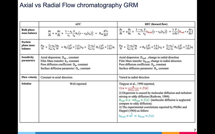
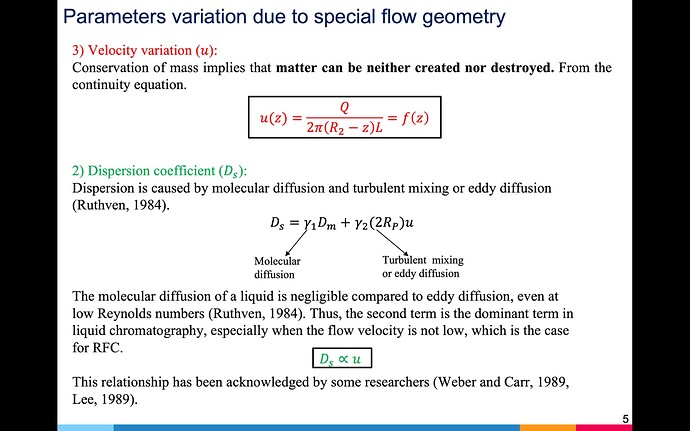
On a different note: The local velocity changes with radial position r as

u = \frac{Q_{in}}{2\pi r L \varepsilon_c} = \frac{v}{r}.

This means that the dispersion coefficient will also change with radius r. What formulas or correlations do we want to support here, @lieres, @j.schmoelder, @all?

3 Likes


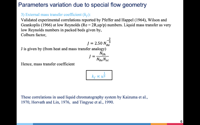
Please have a look, I hope this will help you. If you have any query related to radial chromatography model please ask.

2 Likes

Hey Nadeem,

thanks again for providing the material here! I hope @s.leweke and us will have a chance to talk about this in our next core-dev meeting, next Friday. We will let you know if we have further questions.

In the meantime, it would be great if you could set up a test case in the jupyterhub with some realistic parameters.

1 Like

I will compile that prototype.
Thanks

1 Like