A first prototype of the Colloidal Particle Adsorption (CPA) binding model described by Briskot et al. (2021) has now been implemented in CADET-Core.
It is open for testing, and feedback is highly appreciated  .
.
The detailed set of equations and interface documentation can be found in the feature branch feature/add_CPA_binding_model.
Key Features:
1. Kinetic implementation
The model implements the linear driving force (LDF) formulation for the adsorption kinetics from equation (13) in Briskot et al. (2021):
2. Variable proton concentration (10^{-pH})
- The model requires at least two components: one for the proton concentration and at least one component with (exactly) one binding site.
- The proton concentration is used internally to calculate the pH for the CPA model.
- Since the proton concentration is a state variable, it is possible to define pH profiles via the inlet and couple pH to reactions or other unit operations.
3. Optional salt component
- A salt concentration can be defined to represent dynamic ionic strength.
- If no salt concentration is set, the ionic strength is treated as a model parameter.
- This enables the simulation of salt gradient elution (see below).
Technical implementation details:
1. Internal Newton solver for surface potential \psi_{0,A}
The adsorber surface potential \psi_{0,A} is solved iteratively using a Newton method to balance the surface charge density:
with
- solver tolerance: 10^{-15}(1 + |\psi_{0,A}|)
- max. iterations: configurable via
CPA_MAXITER(default = 100)
2. Model parameters Z_i and \Delta_i
The protein charge can vary with pH; a second-order polynomial is implemented to account for this:
where Z_{i,ref}, pH_{ref}, Z_{i,1}, and Z_{i,2} are model parameters.
Similarly, we have implemented:
with the model parameters \Delta_{i,1} and \Delta_{i,ref}.
Current validation results:
1. Briskot (2021) reproductions
This model reproduces:
-
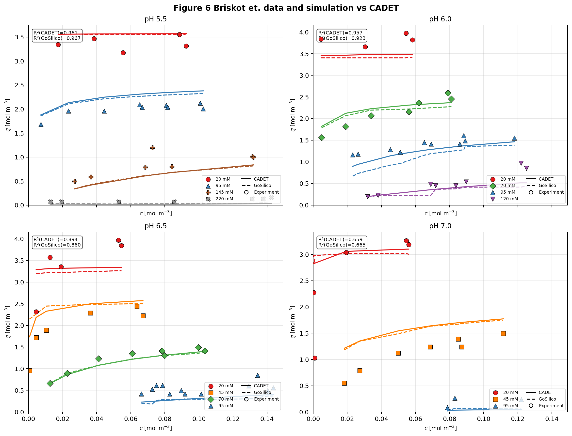
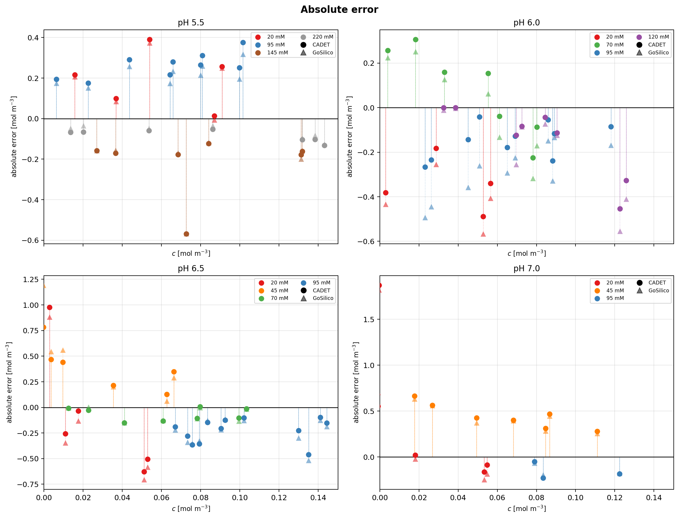
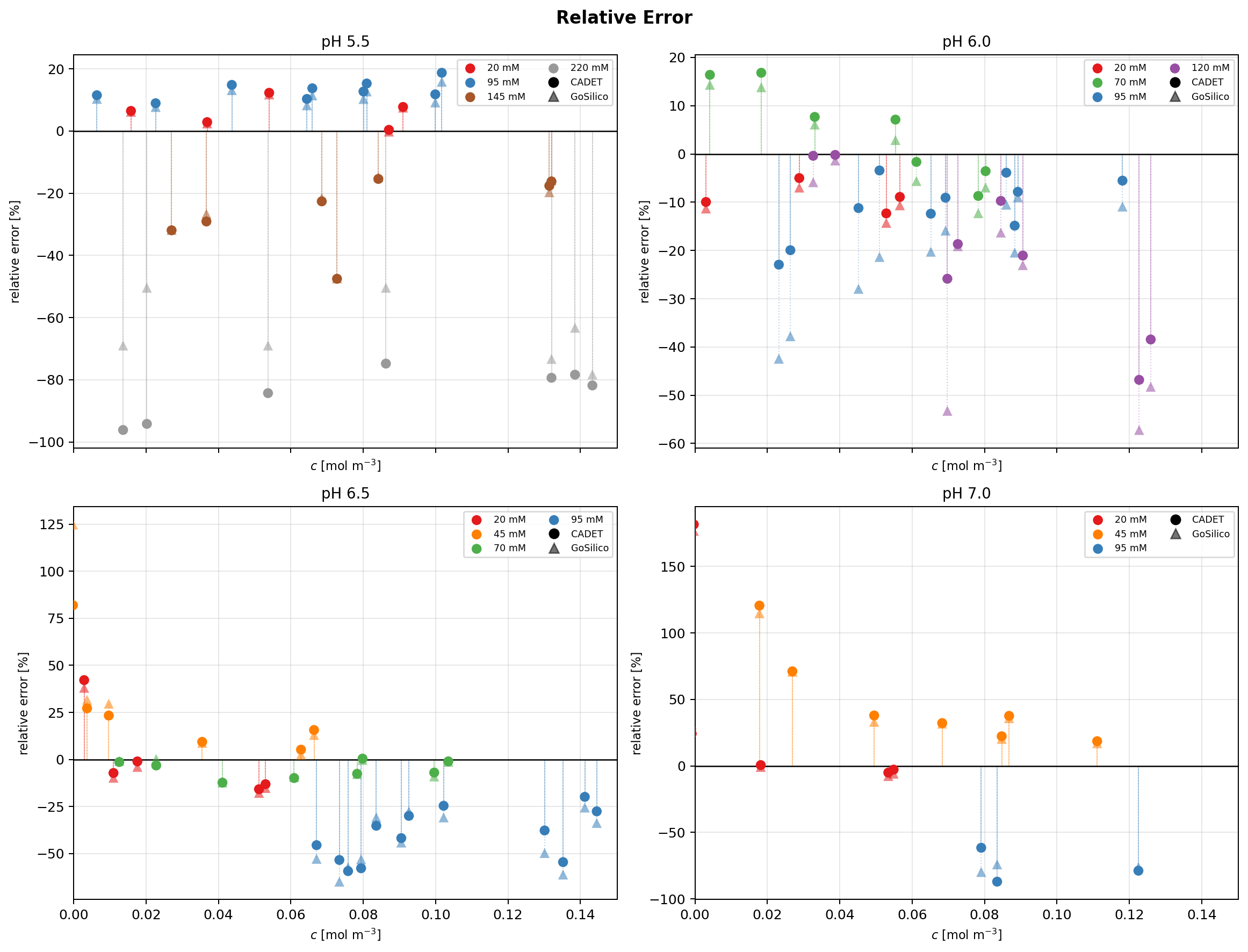
Figure 6 from Briskot et al., Journal of Chromatography A 1653, 462397 (2021), with the following results:
-
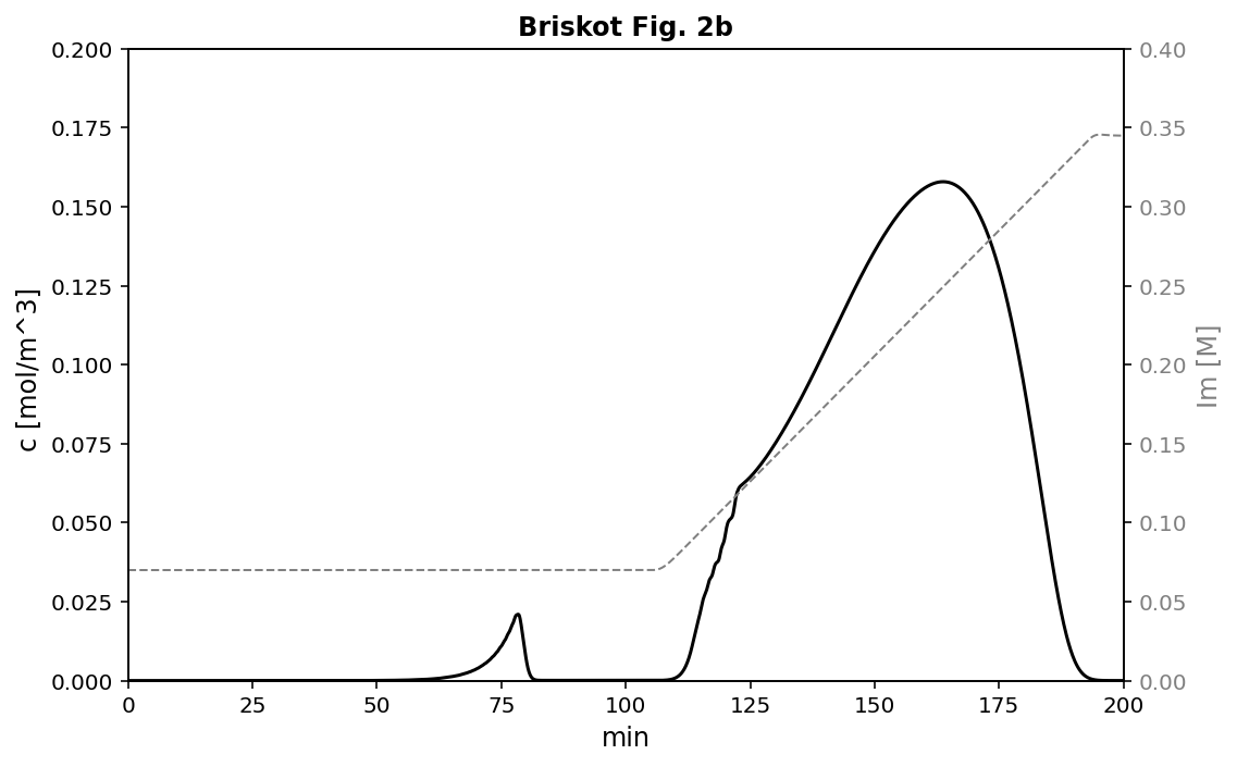
Figure 2b from Briskot et al., Journal of Chromatography A 1654, 462439 (2021), with the following result:


Calculation files to reproduce these results:
Fig2b.py.zip (3.2 KB)
Fig6.py.zip (3.7 KB)
You can see that although the results are similar to those reported in the paper, they are not identical.
For example, in the isotherm results (Fig. 6, Briskot et al.), the final concentrations of q_{v,i} (or c_i^s ) from the CADET and GoSilico simulations vary by between 0.20 and 0.05 absolute difference, and the salt gradient plot appears slightly smoother.
Open Todos
- Steady-state implementation: currently only the dynamic/kinetic model is supported
- CADET-Process support: currently only usable via CADET-Python
- Polynomial degree for Z_i and \Delta_i: currently limited to quadratic
- Diffusion coefficient: currently must be provided via the CPA setup, even though it is already defined in the column parameters