Diverting component streams around CSTR

alters · August 22, 2022, 3:47pm

Hi all,

I am facing some difficulties with implementing a model for the problem I am working on. The goal here is to model the chromatography system as so: inlet model (mIn), gradient mixer CSTR (mCSTR), pre-column tubing PFR (mPFR), column (mCol), outlet model (mOut). In the chromatography system, the gradient buffers are diverted to the mixer and then through the pre-column tubing to the column. However, the protein components bypass the mixer and go straight to the pre-column tubing and the column next. In my unit operation specification (shown below) I would like components 1 and 2 (salt and pH non-binding pseudocomponent) to be routed to the CSTR while the protein components 3 through 8 bypass it. Keep in mind the CADET code for unit operation linkage is written in MATLAB.

% Construct ModelSystem and assign unit operations (order determines IDs)
mSys                       = ModelSystem();
mSys.models          = [mIn, mCSTR, mPFR, mCol, mOut];

% Define valve configurations / unit operation connections
% Valve configuration active on entering section 0
mSys.connectionStartSection = 0;

% Connect unit operations in series 1 (-1 = all ports, all components)
mSys.connections = {[0, 1, -1, -1, -1, -1, ms.flow_rate  ;   ...
                                   1, 2, -1, -1, -1, -1, ms.flow_rate  ;   ...
                                   2, 3, -1, -1, -1, -1, ms.flow_rate  ;   ...
                                   3, 4, -1, -1, -1, -1, ms.flow_rate]};

Above is the starting point I have to build on and create the split component streams around the CSTR. Any help would be appreciated on how to implement this design configuration.

Thanks,
Scott

j.schmoelder · August 22, 2022, 4:14pm

Hey Scott,

In order to specify the component specific connectivity of the network, you have to provide a custom matrix with list of connections in row-major storage.

The columns are structured the following way (see also here):

[UnitOpID from, UnitOpID to, Component from, Component to, volumetric flow rate]

Assuming that the inlet is unit 0, cstr is unit 1, the pfr is unit 2, the column is unit 3, and the outlet is unit 4, it would look something like this:

mSys.connections = {[ ...
    0, 1, 0, 0, flow_rate_1 ; ...
    0, 1, 1, 1, flow_rate_1 ; ...
    1, 2, 0, 0, flow_rate_1 ; ...
    1, 2, 1, 1, flow_rate_1 ; ...
    0, 2, 2, 2, flow_rate_2 ; ...
    0, 2, 3, 3, flow_rate_2 ; ...
    0, 2, 4, 4, flow_rate_2 ; ...
    0, 2, 5, 5, flow_rate_2 ; ...
    0, 2, 6, 6, flow_rate_2 ; ...
    0, 2, 7, 7, flow_rate_2 ; ...
    2, 3, -1, -1, flow_rate_1 + flow_rate_2 ; ...
    3, 4, -1, -1, flow_rate_1 + flow_rate_2 ; ...
]}

Note that you need to assign the corresponding flow rates for the direct connection, as well as the bypass.
Since the Cstr does not “see” all components, you could also reduce n_comp for the unit but in this case, that’s only cosmetic. If you had more complicated unit operations, that might have some numerical advantage.

Let me know if it works!

alters · August 22, 2022, 5:57pm

Hi Johannes,

I am trying this now and will let you know how it goes. One potential issue I see is that the flow rate going into the PFR, column, and outlet in this scheme will be twice what it should be for continuity to be upheld. Does this mean I should double the linear velocity going through these units?

Also, for the method where we reduce the number of components that the CSTR sees: how would we go about implementing this? I was thinking by adding two ports on the inlet model and PFR, but I’m not sure how to configure this.

j.schmoelder · August 23, 2022, 8:04am

You are free to chose any value for the flow rates. The only thing to remember is that for all column units Q_{in} \stackrel{!}{=} Q_{out}. What you can’t do is to just “add” another component to a given unit operation without some kind of flow. But that’s usually unphysical anyway.

Consider this trivial example of two inlets with one component each that connect to an outlet with two components. I’m using Python notation here but conceptually it should be the same in Matlab.

model.root.input.model.unit_000.unit_type = 'INLET'
model.root.input.model.unit_000.ncomp = 1
model.root.input.model.unit_000.inlet_type = 'PIECEWISE_CUBIC_POLY'

model.root.input.model.unit_001.unit_type = 'INLET'
model.root.input.model.unit_001.ncomp = 1
model.root.input.model.unit_001.inlet_type = 'PIECEWISE_CUBIC_POLY'

model.root.input.model.unit_002.unit_type = 'OUTLET'
model.root.input.model.unit_002.ncomp = 2

Now you can map the 0 component of unit_000 to the 0 component of unit_002, and component 0 of unit_001 to the 1 component of unit_002.

model.root.input.model.connections.nswitches = 1
model.root.input.model.connections.switch_000.section = 0
model.root.input.model.connections.switch_000.connections = [
    0, 2, 0, 0, q_0,
    1, 2, 0, 1, q_1,
]

Of course you can also create arbitrarily complicated networks like that.

alters · August 23, 2022, 7:57pm

Hi Johannes,

I am still having an issue and am unsure how to solve it currently.

Below is my systems matrix with the method #1 you suggested (added ports since they are required for the CADET mex). I haven’t tried setting it up with the second method yet.

mSys.connections                        = {[ ...
    0, 1, 0, 0,  0,  0, 0.5*ms.flow_rate   ; ...  % mIn to mCSTR, Comp. 0
    0, 1, 0, 0,  1,  1, 0.5*ms.flow_rate   ; ...  % mIn to mCSTR, Comp. 1
    1, 2, 0, 0,  0,  0, 0.5*ms.flow_rate   ; ...  % mCSTR to mPFR, Comp. 0
    1, 2, 0, 0,  1,  1, 0.5*ms.flow_rate   ; ...  % mCSTR to mPFR, Comp. 1
    0, 2, 0, 0,  2,  2, 0.5*ms.flow_rate   ; ...  % mIn to mPFR, Comp. 2
    0, 2, 0, 0,  3,  3, 0.5*ms.flow_rate   ; ...  % mIn to mPFR, Comp. 3
    0, 2, 0, 0,  4,  4, 0.5*ms.flow_rate   ; ...  % mIn to mPFR, Comp. 4
    0, 2, 0, 0,  5,  5, 0.5*ms.flow_rate   ; ...  % mIn to mPFR, Comp. 5
    0, 2, 0, 0,  6,  6, 0.5*ms.flow_rate   ; ...  % mIn to mPFR, Comp. 6
    0, 2, 0, 0,  7,  7, 0.5*ms.flow_rate   ; ...  % mIn to mPFR, Comp. 7
    2, 3, 0, 0, -1, -1,     ms.flow_rate   ; ...  % mPFR to mCol, Comp. -1 (all)
    3, 4, 0, 0, -1, -1,     ms.flow_rate ]};      % mCol to mOut, Comp. -1 (all)

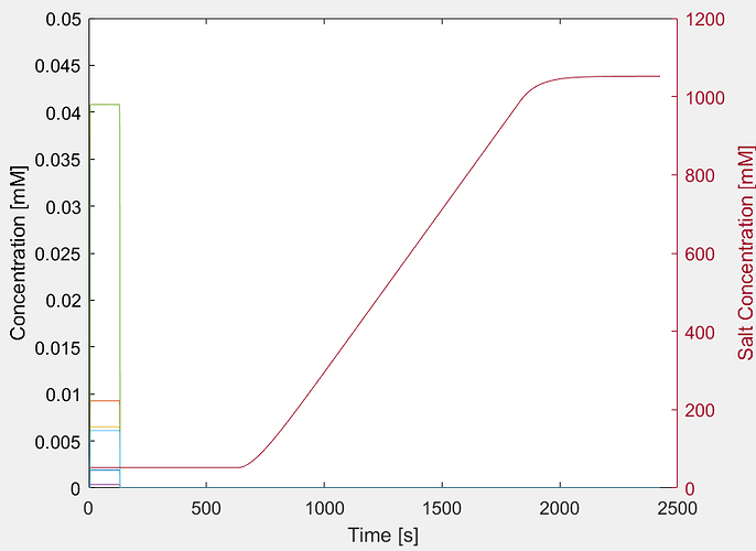
The issue is that the proteins are breaking through 6 seconds into the simulation, which corresponds to the dead time of the tubing PFR. So they are not going into the column. Also, if I increase the SMA parameters to a point where they should definitely be binding (nu = 8, kA = 1, kD = 1, sigma = 100), the simulation crashes right at the end of the loading phase. I am using gIEX for the isotherm model and all the other isotherm parameters are set to zero for this example. The essentially immediate breakthrough can be seen in the LGE outlet profile below.

Would really appreciate it if you can point me in the right direction… I am pretty stuck on this one.

The .m file for the script is attached as well.

bsAbElutionFitGIEX.m (24.0 KB)

EDIT:
I tried changing the number of components for the CSTR to two and linking this appropriately, it actually gives the same connection scheme so I did not need to change that. Unfortunately, the issue with breakthrough still persists. I will also try to use two inlet models instead (one with salt/pH and the other for proteins), but I don’t think this is really fixing the problem - just designing it differently.

j.schmoelder · August 24, 2022, 7:33am

Yes, that’s right. In your case it won’t make much difference. It was just a general remark. For example, if the unit were a column, not having to numerically solve components that aren’t actually present in the column might save some computational time in other situations.

Are you sure you’re plotting the correct unit? In your MATLAB script, you state the following:

	% Extract solution into a matrix with time being the first column
	% Note that we need to extract the outlet of the third unit operation, 
	% which is the OutletModel (order in the ModelSystem matters)
	solution                   = ...
        [result.solution.time, squeeze(result.solution.outlet{3})];

Since MATLAB uses 1-based indexing, don’t you have to use result.solution.outlet{4}?

Unfortunately, I don’t have MATLAB installed so I cannot verify your issue. Please consider using Python since the MATLAB interface is deprecated.

alters · August 25, 2022, 2:41pm

That was the problem!! Thanks a lot Johannes.

alters · September 3, 2022, 6:00pm

Hey Johannes, one follow up question:

I would like to use the same unit operations and connections discussed in this thread, but also use different flow rates in the different sections - load, wash, elution, and strip. I have interstitial velocity as an array of 4x1 containing the velocities during each section and also the film diffusion and axial dispersion being section-dependent. The part I am confused about is how to use different flow rates between the sections. From the CADET manual I found that if the volumetric flow rate and cross sectional area are specified, then the interstitial velocity will be changed accordingly - u = F/(A * eps_c). Since I am not sure how to assign section-dependent flow rate, I think the interstitial velocities are being changed from what I am specifying them as. The only info I could find on having flow rate changing is to use a dynamic flow rate expressed as a polynomial. I would like to simply have a different flow rate in each section, but also ensure that continuity between unit operations is maintained so the simulation runs correctly. I think that this would be easier to use compared to the dynamic flow rate polynomial as far as expressing discontinuous changes in flow rate between sections (e.g., 0.25 * F in load, 0.5 * F in wash, 1 * F in elution, 2 * F in strip).

How can I assign the volumetric flow rates to be section dependent?

j.schmoelder · September 4, 2022, 4:07pm

Hi Scott,

there are two different concepts at play here.

First, it is possible to specify a different flow rate for every section. However, I never use the interstitial velocity to set flow rates and I don’t know if this also works with this approach. I would rather set a diameter for the unit operation and then adjust the volumetric flow rate in the connectivity matrix. Then, the interstitial velocity is simply a function of the flow rate.

Again, I’m not sure how this works with the Matlab interface. In the H5 file, you can specify it the following way:

model.root.input.model.connections.nswitches = 3

model.root.input.model.connections.switch_000.section = 0
model.root.input.model.connections.switch_000.connections = [
    0, 2, 0, 0, q_load,
    1, 2, 0, 1, q_load,
]

model.root.input.model.connections.switch_001.section = 1
model.root.input.model.connections.switch_001.connections = [
    0, 2, 0, 0, q_wash,
    1, 2, 0, 1, q_wash,
]

model.root.input.model.connections.switch_002.section = 2
model.root.input.model.connections.switch_002.connections = [
    0, 2, 0, 0, q_elute,
    1, 2, 0, 1, q_elute,
]

Secondly, it is also possible to describe the flow rate at each section as a piecewise cubic polynomial. For that, you need to enable the CONNECTIONS_INCLUDE_DYNAMIC_FLOW flag. Then, in the connectivity matrix, three more entries are expected per connection row which stand for the const, lin, quad and cubic term. For example, consider a linear increase in flow:

q_const = 0
q_lin = 1e-8 # m³/s²
q_quad  = 0
q_cube = 0

model.root.input.model.connections.connections_include_dynamic_flow = True
model.root.input.model.connections.nswitches = 1
model.root.input.model.connections.switch_000.section = 0
model.root.input.model.connections.switch_000.connections = [
    0, 2, 0, 0, q_const, q_lin, q_quad, q_cube,
    1, 2, 0, 1, q_const, q_lin, q_quad, q_cube,
]
...

alters · September 7, 2022, 12:55am

The first suggestion worked for me! Thanks, Johannes!