Hey everyone,
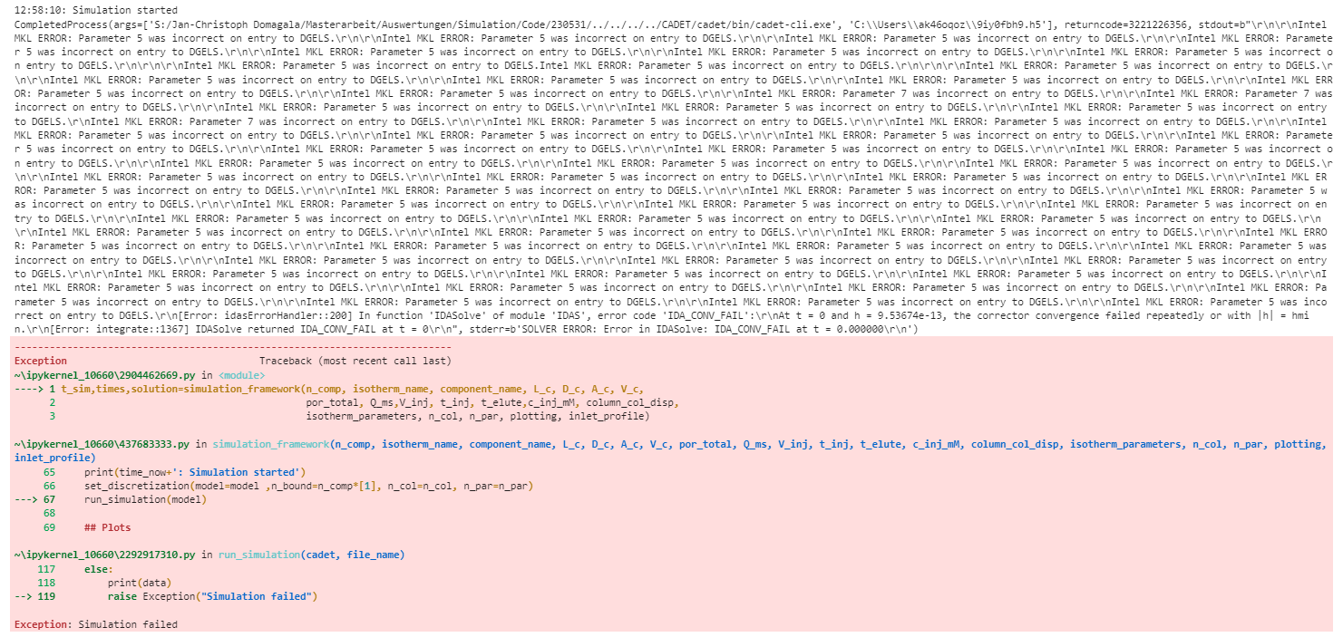
I am runnning into an issue as soon as I change the “is_kinetic” parameter to False or 0.
Is there any condition I am missing in order to use quasi stationary binding?
The function I am using and the error are pasted below.
Thank you in advance for your help!
def simulation_framework(n_comp, isotherm_name, component_name, L_c, D_c, A_c, V_c,
                         por_total, Q_ms,V_inj, t_inj, t_elute,c_inj_mM, column_col_disp,
                         isotherm_parameters, n_col, n_par, plotting, inlet_profile):

    t_start = time.time()

    model = get_cadet_template(n_units=3, split_components_data=False)

    ## Sections
    section_intervals = [t_inj,  t_elute]
    section_times = [0]
    for index, section in enumerate(section_intervals):
        section_times.append(section_times[index] + section) # s

    model.root.input.solver.sections.nsec = len(section_intervals)
    model.root.input.solver.sections.section_times = section_times

    ## Inlet Profile
    model.root.input.model.unit_000.sec_000.const_coeff = c_inj_mM
    model.root.input.model.unit_000.sec_001.const_coeff = [0]*n_comp

    # set the times that the simulator writes out data for
    model.root.input.solver.user_solution_times = np.linspace(0,  t_inj+  t_elute, 10001)

    ## Flowsheet
    # INLET
    model.root.input.model.unit_000.unit_type = 'INLET'
    model.root.input.model.unit_000.ncomp = n_comp
    model.root.input.model.unit_000.inlet_type = 'PIECEWISE_CUBIC_POLY'

    # Column
    model.root.input.model.unit_001.unit_type = 'LUMPED_RATE_MODEL_WITHOUT_PORES'
    model.root.input.model.unit_001.ncomp = n_comp
    model.root.input.model.unit_001.col_length = L_c
    model.root.input.model.unit_001.total_porosity = por_total
    model.root.input.model.unit_001.col_dispersion = column_col_disp
    model.root.input.model.unit_001.cross_section_area = A_c

    kA=isotherm_parameters[0]
    kD=isotherm_parameters[1]
    q_max=isotherm_parameters[2]

    model.root.input.model.unit_001.adsorption_model = 'MULTI_COMPONENT_LANGMUIR'
    model.root.input.model.unit_001.adsorption.is_kinetic = 0
    model.root.input.model.unit_001.adsorption.mcl_kA = kA
    model.root.input.model.unit_001.adsorption.mcl_kD = kD
    model.root.input.model.unit_001.adsorption.mcl_qmax = q_max
    model.root.input.model.unit_001.init_c = [0]*n_comp
    model.root.input.model.unit_001.init_q = [0]*n_comp

    ## Outlet
    model.root.input.model.unit_002.unit_type = 'OUTLET'
    model.root.input.model.unit_002.ncomp = n_comp

    ## Switches and connections
    model.root.input.model.connections.nswitches = 1
    model.root.input.model.connections.switch_000.section = 0
    model.root.input.model.connections.switch_000.connections = [0, 1, -1, -1, Q_ms,
                                                                 1, 2, -1, -1, Q_ms
                                                                  ]

    ## Run simulation
    now2 = datetime.now()
    time_now = now2.strftime("%H:%M:%S")
    print(time_now+': Simulation started')
    set_discretization(model=model ,n_bound=n_comp*[1], n_col=n_col, n_par=n_par)
    run_simulation(model)

    ## Plots
    added_input_solutions = [0]* len(model.root.output.solution.unit_000.solution_outlet[:,0])
    added_output_solutions = [0]* len(model.root.output.solution.unit_002.solution_outlet[:,0])
    for i3 in range(n_comp):
        added_input_solutions = added_input_solutions+model.root.output.solution.unit_000.solution_outlet[:,i3]*M[i3]/1000
        added_output_solutions = added_output_solutions+model.root.output.solution.unit_002.solution_outlet[:,i3]*M[i3]/1000


    if plotting ==True:
        fontsize=12
        figsize=[25,12]
        fig3, ax3 = plt.subplots(figsize=cm2inch(figsize[0], figsize[1]), dpi=120)
        ax3.tick_params(axis='x', labelsize=fontsize)
        ax3.tick_params(axis='y', labelsize=fontsize)
        if inlet_profile == True:
            ax3.plot(model.root.output.solution.solution_times/60, added_input_solutions, 'k', label=component_name +'combined simulated inlet' )

        for i2 in range(n_comp):
            ax3.plot(model.root.output.solution.solution_times/60, model.root.output.solution.unit_002.solution_outlet[:,i2]*M[i2]/1000, color=colors[i2])

        ax3.plot(model.root.output.solution.solution_times/60, added_output_solutions, 'k--', label=component_name+' 15-30 combined simulated outlet')
        ax3.set_xlabel('Time (min)',fontsize=fontsize)
        ax3.set_ylabel(component_name + ' concentration (g/L)',fontsize=fontsize)

        lines, labels = ax3.get_legend_handles_labels()

        #ax3.legend(lines, labels,bbox_to_anchor=(1.13, 1),loc='upper left', borderaxespad=0)
        ax3.legend(lines, labels,fontsize=fontsize)
        #plt.subplots_adjust(right=0.7)
        plt.tight_layout()

    t_end = time.time()
    t_sim = format(round(t_end - t_start,1))
    print('Simulation duration =',t_sim,'seconds')

    return t_sim, model.root.output.solution.solution_times/60, added_output_solutions