Factoring in the porosity distribution for adsorption capacity

As far as I know particle porosity has an inverse proportion to the adsorption capacity of a particle due to how CADET is coded.
So an increase in particle porosity, which should mean a higher capacity due to more surface area inside the particle, would lead to a decrease in capacity in CADET simulations.

The question for me is how do I correct this in my model setup.

At the moment I am using a Gaussian distribution as basis for my porosity distribution.
With a homogeneous particle distribution inside the column this is not a issue, but I am also adding using position distributions. This means that my adsorption capacity is a function that is based on the particle capacities at column height x.

In the following test case I look at 3 columns:

c_feed = [10]                  
n_bound = [1]            
t_in_seconds =300000*60                       
n_col= 4
volume_flow_rate = 4.71e-5  

resolution = int(t_in_seconds/60)
adsorption_parameters = Dict()
adsorption_parameters.is_kinetic = 1
adsorption_parameters.FLDF_KKIN = [1]                            
adsorption_parameters.FLDF_KF = [41312.942982]             
adsorption_parameters.FLDF_N = [2.092987]   
k_film = [1]    
porediffusion= [1] 
k_RL = [0]

Reference column (blue):

sizeclasses= 1.25/2000
porosityclasses= 0.455
n_partype=1
vol_frac =1

Green graph (low porosity at the top)

sizeclasses= [1.25/2000,1.25/2000] 
porosityclasses= [0.355,0.555]
n_partype=2
vol_frac =[1,0,1,0,0,1,0,1]

Red graph (high porosity at the top)

sizeclasses= [1.25/2000,1.25/2000] 
porosityclasses= [0.355,0.555]
n_partype=2
vol_frac =[0,1,0,1,1,0,1,0]

image

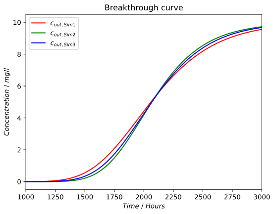
As mentioned before the graph (green) with a low porosity at the beginning/top of the column has a later initial breakthrough which would mean a higher adsorption capacity in the top part of the column.
One can also see that this effect does not seem symmetric.

Now for my case with a Gaussian distribution my Idea would be to mirror the volume fractions inside my column because the porosity distribution is symmetrical at the mean value.

Since my testcase I am not sure anymore if this approach is a valid correction.
So my question would be how I can adjust this issue numerically in my model setup for symmetrical and non-symmetrical porosity distributions.

Hello,

I cant answer all of your questions, but I would like to add some thoughts on this.
Firstly, an increase in porosity does not always increase the surface area/capacity of a particle, it might can also decrease the surface area.
If you want to compare the total capacity of your columns you need to calculate the area above the curve and not when the breakthrough arises (which is the dynamic binding capacity) as the shape of the breakthrough can be influence by many parameters. Looking at your breakthrough curves, the systems seem to have the same capacity. For example the red curve start to break though earlier, but after the inflection point the signal is below the other curves.

An explanation for the deviation between red an green might be that if you change the porosity this will also change the phase ratio. This will change the equilibrium between your mobile and stationary phase.

I hope this helps.

Best

1 Like

Thank you for the input Lukas.

It might not have been well described by myself, but I am not looking at the total capacity of column.
Since I am using more than one particle type I have to define where a particle is and therefore influence the breakthrough curve solely by position. Based on your comment it seems I am looking at the dynamic binding capacity.

Your explanation of the phase ratio change is something I am not familiar with.
Could you elaborate that further?

Hello,

if you take a look at the model equations (e.g. Lumped rate model without pores (LRM) — CADET) there is always the variable beta which accounts for the phase ratio. Basically how much of your column is stationary phase and how much is mobile phase. This will obviously change if you change the porosity, as it is calculated from the porosities.

The phase ratio is important to calculate the transfer of a molecule from the mobile phase to the stationary phase and vice versa. The binding models only correlate the concentration in the stationary phase with the concentration mobile phase. In an extreme case with basically no stationary phase (porosity approaching 1) there will be no binding to the stationary phase irrespectively how strong the binding is.

2 Likes

Thanks for the explanation.

My model as well as the tests above use the General Rate Model. The GRM only defines a column phase ratio:
image
General Rate Model: Phase Ratio

The phase ratio in that case is only dependent on the column porosity which is constant for the example above.
Other than that I don’t see a direct correlation between phase ratio and the results in testcases.

No, the one you showed is the column phase ratio (index c). But there is another phase ratio for the particles in eq. 4, although we do not explicitly call it that.

\beta_p = \frac{\varepsilon_p}{1-\varepsilon_p}

Edit: Updated the equation.

So the difference between the green and the red graph in my example could be happening in part due to the phase ratio, which is nonlinear.

Then I would need a clarification from @lieres or @j.schmoelder in what way the porosity influences the adsorption capacity of the particle.
Since it is possible it increases or decreases it, the question is how does it work in CADET?

We assume a constant volume specific capacity; i.e. the number of binding sites per unit volume of stationary phase. If you have more volume of stationary phase, you also get more capacity. That’s a linear (!) relationship.

This volume obviously changes if you change the porosities. The column phase ratio gives you the ratio of liquid phase to solid phase; the pore phase ratio the ratio of particle liquid (i.e. the pore volume) and particle solid (i.e. the stationary phase volume).

Thanks for the explanation.

So for the example above:
Increasing the porosity by 22% (0.1/0.455) to 0.555 would mean a 22% decrease in the particle capacity because the stationary phase is (1-porosity). Since the correlation is linear the inverse would happen if the porosity decreases.

At the same time the phase ratio which effects the mass balance in CADET (Eq. 4 in GRM) would increase by almost 50% with a porosity increase of 0.1.

beta(porosity = 0.455) =0.835
beta(porosity = 0.555) =1.247

On the other-hand a decrease of the porosity by 0.1 would decrease the phase ratio by only 34%

beta(porosity = 0.455) =0.835
beta(porosity = 0.355) =0.550

As stated by Lukas the phase ration seems to be the reason that the green and red graph are not symmetrical around the blue reference case.

For my application:
I want the increase in porosity in my model to mean that the stationary volume also increases so that my capacity increases accordingly.
This can not be done with the porosity value because that would also influence the phase ratio in a non desirable way.

Is there a way to influence the stationary phase volume without effecting the phase ratio parameter?

I don’t think it’s possible to influence the stationary phase volume without affecting the phase ratio. Also, which porosity are you talking about?

If I understand you correctly, to keep the overall capacity constant (w.r.t. total column volume), you want to correct its value s.t. it counters the changes of the porosities, correct?

Maybe thinking about the definition of porosities helps to better understand what happens when you change their values.

V_c = V_p + V_b
V_b = \varepsilon_c \cdot V_c \\ V_p = (1 - \varepsilon_c) \cdot V_c

and

V_p = V_l + V_s
V_l = \varepsilon_p \cdot V_p \\ V_s = (1 - \varepsilon_p) \cdot V_p

with:

  • V_c Total column (cylinder) volume
  • V_b Interstitial (bulk) volume
  • V_p Total particle volume
  • V_l Particle liquid volume
  • V_s Particle solid volume

Now you could think of the capacity \Lambda as

\Lambda = a \cdot V_s

Where a is some parameter that gives you information about the number of binding sites per unit volume stationary phase.

Hope that helps.

Edit: Please take that equation with parameter a with a grain of salt. I need to think about the units. It’s just to give you a rough idea of how I would approach this issue.

Based on this equation the total column capacity formula would be:

Λ=a*(1-ε_p)*(1-ε_c)*V_c

So increasing the particle porosity decreases the overall capacity with everything else constant.

With the discretization of the column V_c = sum(V_c_k) for k in range(ncol),
we also get the discretization of the capacity Λ =sum(Λ_k) for k in range(ncol).

For ncol= 2
V_c_1=V_c_2

ε_p1=0.3
Λ1=a*(1-ε_p1)*(1-ε_c)*V_c_1

ε_p2=0.5
Λ2=a*(1-ε_p2)*(1-ε_c)*V_c_2
with  Λ2 < Λ1 despite ε_p2 > ε_p1

The goal would be to achieve Λ2 > Λ1 in proportion to ε_p2 > ε_p1.
This would only be possible by changing parameter a.

Sorry for the bad formatting, not sure how you did it.

In CADET, the ionic capacity \Lambda and the stationary phase concentration q_i are defined per particle solid volume V_s and the pore phase concentration c_i is defined per particle liquid volume V_l. It is important to understand that through these definitions, the values of the adsorption and desorption constants k_{a,i} and k_{d,i} implicitly depend on the particle porosity \varepsilon_p.

The the ionic capacity can alternatively be defined per total particle volume V_p, and this value will not depend on \varepsilon_p. Let’s denote it \hat{\Lambda}. This value needs to be converted to \Lambda = \frac{V_p}{V_s} \hat{\Lambda} when being used in CADET.

Let’s introduce \hat{q}_i, \hat{c}_i, \hat{k}_{a,i} and \hat{k}_{d,i} all defined per V_p. The SMA model reads:

\frac{dq_i}{dt} = k_{a,i} c_i \bar{q}_0^{\nu_i} - k_{d,i} q_i c_0^{\nu_i}

Now, convert q_i and c_i:

\frac{V_s}{V_p} \frac{d\hat{q}_i}{dt} = k_{a,i} \frac{V_l}{V_p} \hat{c}_i \frac{V_s^{\nu_i}}{V_p^{\nu_i}} \hat{\bar{q}}_0^{\nu_i} - k_{d,i} \frac{V_s}{V_p} \hat{q}_i \frac{V_l^{\nu_i}}{V_p^{\nu_i}} \hat{c}_0^{\nu_i}

Collect terms

\frac{d\hat{q}_i}{dt} = \frac{V_p}{V_s} \frac{V_l}{V_p} \frac{V_s^{\nu_i}}{V_p^{\nu_i}} k_{a,i} \hat{c}_i \hat{\bar{q}}_0^{\nu_i} - \frac{V_p}{V_s} \frac{V_s}{V_p} \frac{V_l^{\nu_i}}{V_p^{\nu_i}} k_{d,i} \hat{q}_i \hat{c}_0^{\nu_i}

Simplify:

\frac{d\hat{q}_i}{dt} = \frac{V_l V_s^{\nu_i-1}}{V_p^{\nu_i}} k_{a,i} \hat{c}_i \hat{\bar{q}}_0^{\nu_i} - \frac{V_l^{\nu_i}}{V_p^{\nu_i}} k_{d,i} \hat{q}_i \hat{c}_0^{\nu_i}

Conclude:

\frac{d\hat{q}_i}{dt} = \hat{k}_{a,i} \hat{c}_i \hat{\bar{q}}_0^{\nu_i} - \hat{k}_{d,i} \hat{q}_i \hat{c}_0^{\nu_i}

with \hat{k}_{a,i} = \frac{V_l V_s^{\nu_i-1}}{V_p^{\nu_i}} k_{a,i} and \hat{k}_{d,i} = \frac{V_l^{\nu_i}}{V_p^{\nu_i}} k_{d,i}, or k_{a,i} = \frac{V_p^{\nu_i}}{V_l V_s^{\nu_i-1}} \hat{k}_{a,i} and k_{d,i} = \frac{V_p^{\nu_i}}{V_l^{\nu_i}} \hat{k}_{d,i}.

The impact of \nu_i might look bizarre at the first glance but is due to the definition of the SMA model. Since the values of \hat{\Lambda}, \hat{k}_{a,i} and \hat{k}_{d,i} do not depend on \varepsilon_p, they can be used as “reference” from which the values of \Lambda, k_{a,i} and k_{d,i} can be deduced for different \varepsilon_p.

With all these transforms correctly applied, \varepsilon_p should not impact binding. The approach can also be helpful to compare and adjust the values of k_{a,i} and k_{d,i} when changing the characteristic charge \nu_i.

On a side note, the whole procedure can be simplified by introducing reference concentrations q_{ref} and c_{ref}.

2 Likes

Do you mean that changing \varepsilon_p should not affect binding affinity, or not affect binding capacity, or not affect either?

There are some interesting implications on binding capacity here as \varepsilon_p \rightarrow 1

Defining total porosity

\varepsilon_t = \varepsilon_c + \left(1-\varepsilon_c\right)\varepsilon_p

If \varepsilon_p = 1, ~\varepsilon_t = 1

Defining solid phase volume; V_s is the solid phase volume and V_c is the total column volume

V_s = (1-\varepsilon_t)V_c

Therefore,

V_s = 0 when \varepsilon_p = 1

Defining ionic capacity per solid phase volume; \Lambda_c is the ionic capacity per entire column volume and \Lambda_s is per solid phase volume

\Lambda_s = \Lambda_c \frac{V_c}{V_s}

Accordingly,

\Lambda_s = \frac{\Lambda_c}{1-\varepsilon_t}

Therefore,

\displaystyle \lim_{\varepsilon_p\to 1} \Lambda_s=\infty

Defining saturation capacity q_{max} in the SMA model

q_{max} = \frac{\Lambda_s}{\nu + \sigma}

Therefore,

\displaystyle \lim_{\varepsilon_p\to 1} q_{max,s}=\infty

Here, q_{max,s} refers to the saturation capacity on a solid phase volume basis.

Redefining saturation capacity volume basis,

q_{max,c} = q_{max,s}\left(\frac{V_s}{V_c}\right)

Accordingly,

q_{max,c} = q_{max,s}\left(1-\varepsilon_t\right)

Therefore,

\displaystyle \lim_{\varepsilon_p\to 1} q_{max,c}=\infty

It should be noted that the definition of \Lambda_s is confounding because \Lambda_c must be zero if there is no stationary phase for ions to bind to. Therefore, the above steps may not be correct.

Going back to the earlier point…

My intuition tells me that binding affinity and capacity on a V_c basis should not change when increasing \varepsilon_p because \Lambda_s changes accordingly. However, this seems to contradict the above analysis, namely that \lim_{\varepsilon_p\to 1} q_{max,c}=\infty.

How do we resolve this contradiction?

OK, I should have stated more carefully that moderate changes in the model parameter \varepsilon_p do not change either capacity of affinity when defined per V_p. This concept can be useful when the binding properties are determined independently of the porosity and the porosity is determined later. The limiting case \varepsilon_p \rightarrow \infty creates a mathematical singularity that I would consider practically irrelevant as the ionic binding sites do of course need to be located in some physically existing stationary phase.

I fully agree with your intuition.

1 Like