Hello Sean,
thanks again for stopping by the Office Hours yesterday! I’ve had some time to mull things over and have two working solutions. Well, at least I hope I do.
First solution:
using the Mobile Phase Modulator Langmuir Isotherm.
It uses this equation:
\frac{\mathrm{d} q_i}{\mathrm{d} t} = k_{a,i} e^{\gamma_i c_{p,0}} c_{p,i}\: q_{\text{max},i} \left( 1 - \sum_{j=1}^{N_{\text{comp}} - 1} \frac{q_j}{q_{\text{max},j}} \right) - k_{d,i} \: c_{p,0}^{\beta_i} \: q_i
with the assumption, that the 0-th component c_{p,0} is some adsorption-modifying component, in our case, the acid HNO3.
If I understand your calculation for kEq (via k_prime) correctly:
k_prime_value = k_prime[element]['constant'] * (M_HNO3 ** k_prime[element]['slope']
or simplified to
kEq = k_prime*1.75 = ['constant'] * 1.75 * (M_HNO3 ** ['slope'])
we can use the MPML isotherm to model that behavior. First, because we do not consider kinetic effects, we assume that \frac{\mathrm{d} q_i}{\mathrm{d} t} =0. Then, by dividing the isotherm by c_{p,0}^{\beta_i} we get
c_{p,0}^{-\beta_i}\frac{\mathrm{d} q_i}{\mathrm{d} t} = 0 = k_{a,i}\: c_{p,0}^{-\beta_i} \:e^{\gamma_i c_{p,0}} c_{p,i}\: q_{\text{max},i} \left( 1 - \sum_{j=1}^{N_{\text{comp}} - 1} \frac{q_j}{q_{\text{max},j}} \right) - k_{d,i} \: q_i
So k_{a,i} takes the place of the “constant”, -\beta_i takes the place of “slope” and c_{p,0} is the concentration of HNO3. (and we set \gamma_i =0, as we do not need that influence).
I have a working example with only CADET-Process below. (I’ve taken the liberty to change some data storage code during the debugging to make tracing values easier for me)
import os
from CADETProcess.processModel import ComponentSystem, MobilePhaseModulator
from CADETProcess.processModel import Inlet, LumpedRateModelWithPores, Outlet
from CADETProcess.processModel import FlowSheet
from CADETProcess.processModel import Process
from CADETProcess.simulator import Cadet
# Derived Constants
CADET_CLI_PATH = os.path.join(os.path.abspath('.'), 'CADET/install')
assert os.path.exists(CADET_CLI_PATH), f"CADET_CLI_PATH doesn't exist: {CADET_CLI_PATH}"
WORKING_FOLDER = os.path.join(os.path.abspath('.'), 'ln-1_model')
# A few variables to simplify variations on the theme I wanted to be able to generate.
load = 150. # Used 150 and 10
column_length_multiplier = 1 # Used 1 and 3
run_length_multiplier = 1 # Used 1 and 5
# Simplified Binding Isotherms:
k_prime = {
'La': {'constant': 0.05641268710558851, 'slope': -2.620012417528447},
'Nd': {'constant': 0.16512886791167147, 'slope': -2.6425049824718645},
'Eu': {'constant': 0.6698847949281866, 'slope': -3.2578698806430073},
}
# Process Information - Used to create process events later
load_comp = [load, load, load] # mMol/L = mol/m^3
initial_flowrate = 7 / 5 / 60 / 1e6 # 7mL / 5min / 60sec/min / 1e6mL/m^3 = m^3/s
load_flowrate = initial_flowrate
acid_load_concentration = 0.01 # mol / L # ToDO: convert to mol / m^3 and adjust slope parameters
acid_elution_concentration = 0.5 # mol / L # ToDO: convert to mol / m^3 and adjust slope parameters
# load_profile: ([HNO3] in M, vol in ml, step name)
load_profile = [
{"acid": acid_load_concentration, "volume": 0.99, "name": "load"},
{"acid": acid_load_concentration, "volume": 2, "name": "rinse1"},
{"acid": acid_load_concentration, "volume": 2, "name": "rinse2"},
{"acid": acid_load_concentration, "volume": 2, "name": "rinse3"},
] # (diluent acid conc [M], vol [mL], name)
elute_flowrate = 5 / 40 / 60 / 1e6 # 5mL / 40min / 60sec/min / 1e6mL/m^3 = m^3/s
# Gradient steps: ([HNO3] in M, vol in ml, flowrate in m^3/s)
acid_profile = [
{"acid": acid_load_concentration, "volume": 5, "flowrate": elute_flowrate},
{"acid": acid_elution_concentration, "volume": 5, "flowrate": elute_flowrate},
] # (acid conc (M), vol (mL), flow rate (m^3/s))
# Create a list of each section's HNO3 molarity:
section_acid_concentrations = [step["acid"] for step in load_profile] + [step["acid"] for step in acid_profile]
##########################################################
# Initial CADET-process Simulation Specification
# Component System
component_system = ComponentSystem(["HNO3", 'La', 'Nd', 'Eu'])
# Binding Model
binding_model = MobilePhaseModulator(component_system, name='MPM')
binding_model.is_kinetic = False
binding_model.adsorption_rate = [0] + [k_prime[element]["constant"] * 1.75 for element in ['La', 'Nd', 'Eu']]
binding_model.desorption_rate = [1] * component_system.n_comp
binding_model.capacity = [160] * component_system.n_comp # mol/m^3
binding_model.ion_exchange_characteristic = [0] + [-1 * k_prime[element]["slope"] for element in ['La', 'Nd', 'Eu']]
binding_model.hydrophobicity = [0] * component_system.n_comp
binding_model.bound_states = [0, 1, 1, 1]
# Verify that the binding model has all required parameters:
assert binding_model.check_required_parameters()
# Unit Operations
inlet = Inlet(component_system, name='inlet')
inlet.flow_rate = initial_flowrate
# Column based on LumpedRateModelWithPores
column = LumpedRateModelWithPores(component_system, 'column')
column.binding_model = binding_model
column.length = 0.0408 * column_length_multiplier # m = 4.08 cm times multiplier
column.diameter = 0.008 # m = 0.8 cm Dia
column.bed_porosity = 0.67 # 0 to 1 - Porosity of the bed
column.particle_radius = 7.5e-5 # m = 75 microns bead size
column.particle_porosity = 0.16 # 0 to 1 - Porosity of particles
column.axial_dispersion = 2.0e-7 # Dispersion rate of components in axial direction
column.film_diffusion = 1.0e-2 # Diffusion rate for components in pore volume. m/s
column.q = [0., 0., 0.] # mol/m^3 # q (bound concentration) only has three entries because the acid does not bind
column.c = [0.01, 0., 0., 0.] # mol/m^3 # The column is conditioned with 0.01 M HNO3.
column.cp = [0.01, 0., 0., 0.] # mol/m^3 # The column is conditioned with 0.01 M HNO3.
outlet = Outlet(component_system, name='outlet')
# Flow Sheet
flow_sheet = FlowSheet(component_system)
flow_sheet.add_unit(inlet)
flow_sheet.add_unit(column)
flow_sheet.add_unit(outlet)
flow_sheet.add_connection(inlet, column)
flow_sheet.add_connection(column, outlet)
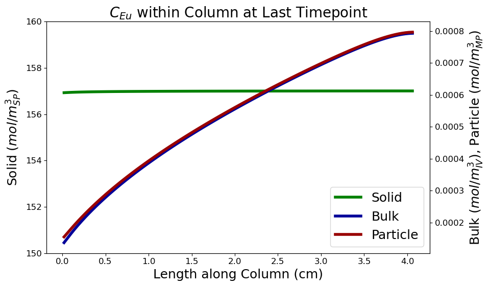
# Record the column particle solution.
column.solution_recorder.write_solution_particle = True
column.solution_recorder.write_solution_bulk = True
column.solution_recorder.write_solution_solid = True
# Define CADET Process Events
process = Process(flow_sheet, 'LN-1')
# Load and Triple Rinse:
t = 0
conc = load_comp
process.add_event(f"Start", 'flow_sheet.inlet.flow_rate', initial_flowrate, t)
for event in load_profile:
if event["name"] != 'load':
conc = [conc[i] * 0.01 / event["volume"] for i in
range(3)] # 1% left in container diluted in vol ml
process.add_event(event["name"], 'flow_sheet.inlet.c', [event["acid"], ] + conc, t)
t += event["volume"] * 1e-6 / initial_flowrate
# Gradient
flowrate = elute_flowrate
process.add_event("elute_start", 'flow_sheet.inlet.flow_rate', flowrate, t)
n = 0
# Loop over acid concentration steps:
for event in acid_profile:
if event["flowrate"] != flowrate:
n += 1
flowrate = event["flowrate"]
process.add_event(f"flow_adj_{n}", 'flow_sheet.inlet.flow_rate', flowrate, t)
process.add_event(
name=f"acid_conc_{str(event['acid']).replace('.', '_')}",
parameter_path='flow_sheet.inlet.c',
state=[event["acid"], 0, 0, 0],
time=t
)
t += event["volume"] * 1e-6 / flowrate
process.cycle_time = t * run_length_multiplier
process_simulator = Cadet()
sim_results = process_simulator.simulate(process)
sim_results.solution.outlet.outlet.plot()
Second solution:
External functions.
This covers 90% of the application, however, it does not yet accept different external functions for the different components. So all components are modified by the same external function.
#!~/.conda/envs/cadet/bin/python
import numpy as np
import os
import matplotlib.pyplot as plt
import scipy.integrate as integrate
from CADETProcess.processModel import ComponentSystem
from CADETProcess.processModel import Langmuir
from CADETProcess.processModel import Inlet, LumpedRateModelWithPores, Outlet
from CADETProcess.processModel import FlowSheet
from CADETProcess.processModel import Process
from CADETProcess.simulator import Cadet
# Derived Constants
# CADET_CLI_PATH = os.path.join(os.path.abspath('.'), 'CADET/install')
# assert os.path.exists(CADET_CLI_PATH), f"CADET_CLI_PATH doesn't exist: {CADET_CLI_PATH}"
WORKING_FOLDER = os.path.join(os.path.abspath('.'), 'ln-1_model')
# A few variables to simplify variations on the theme I wanted to be able to generate.
load = 0. # Used 150 and 10
column_length_multiplier = 1 # Used 1 and 3
run_length_multiplier = 1 # Used 1 and 5
# Simplified Binding Isotherms:
k_prime = {
'La': {'constant': 0.05641268710558851, 'slope': -2.620012417528447},
'Nd': {'constant': 0.16512886791167147, 'slope': -2.6425049824718645},
'Eu': {'constant': 0.6698847949281866, 'slope': -3.2578698806430073},
}
def k_prime_func(element: str, M_HNO3: float) -> float:
"""Returns retention factor (k') for LN Resin as a function of [HNO3] in M.
Args:
element (str): 2 letter symbol for element
M_HNO3 (float): Concentration of Nitric Acid [HNO3] in molarity (M)
Returns:
float: k' or Retention factor (formerly known as capacity factor) of the material
on LN Resin (HDEHP stationary phase) as a function of [HNO3] in M.
"""
return max(1., round(k_prime[element]['constant'] * (M_HNO3 ** k_prime[element]['slope']), 5))
# Process Information - Used to create process events later
load_comp = [load, load, load] # mMol/L = mol/m^3
initial_flowrate = 7 / 5 / 60 / 1e6 # 7mL / 5min / 60sec/min / 1e6mL/m^3 = m^3/s
load_flowrate = initial_flowrate
# load_profile: ([HNO3] in M, vol in ml, step name)
load_profile = [
(0.01, 0.99, "load"),
(0.01, 2, "rinse1"),
(0.01, 2, "rinse2"),
(0.01, 2, "rinse3"),
] # (diluent acid conc [M], vol [mL], name)
elute_flowrate = 5 / 40 / 60 / 1e6 # 5mL / 40min / 60sec/min / 1e6mL/m^3 = m^3/s
# Gradient steps: ([HNO3] in M, vol in ml, flowrate in m^3/s)
acid_profile = [
(0.01, 5, elute_flowrate),
(0.5, 5, elute_flowrate)
] # (acid conc (M), vol (mL), flow rate (m^3/s))
# Create a list of each section's HNO3 molarity:
section_acid_concentrations = [step[0] for step in load_profile] + [step[0] for step in acid_profile]
# Initial CADET-process Simulation Specification
# Component System
component_system = ComponentSystem(['La', 'Nd', 'Eu'])
# Binding Model
binding_model = Langmuir(component_system, name='langmuir')
binding_model.is_kinetic = False
# The column is conditioned with 0.01 M HNO3.
binding_model.adsorption_rate = [k_prime_func(component.name, 0.01) * 1.75 for component in component_system]
binding_model.desorption_rate = [1] * component_system.n_comp
binding_model.capacity = [160] * component_system.n_comp # mol/m^3
# Verify that the binding model has all required parameters:
assert binding_model.check_required_parameters()
# Unit Operations
inlet = Inlet(component_system, name='inlet')
inlet.flow_rate = initial_flowrate
# Column based on LumpedRateModelWithPores
column = LumpedRateModelWithPores(component_system, 'column')
column.binding_model = binding_model
column.length = 0.0408 * column_length_multiplier # m = 4.08 cm times multiplier
column.diameter = 0.008 # m = 0.8 cm Dia
column.bed_porosity = 0.67 # 0 to 1 - Porosity of the bed
column.particle_radius = 7.5e-5 # m = 75 microns bead size
column.particle_porosity = 0.16 # 0 to 1 - Porosity of particles
column.axial_dispersion = 2.0e-7 # Dispersion rate of components in axial direction
column.film_diffusion = 1.0e-2 # Diffusion rate for components in pore volume. m/s
column.q = [10., ] * component_system.n_comp # mol/m^3
outlet = Outlet(component_system, name='outlet')
# Flow Sheet
flow_sheet = FlowSheet(component_system)
flow_sheet.add_unit(inlet)
flow_sheet.add_unit(column)
flow_sheet.add_unit(outlet)
flow_sheet.add_connection(inlet, column)
flow_sheet.add_connection(column, outlet)
# Record the column particle solution.
column.solution_recorder.write_solution_particle = True
column.solution_recorder.write_solution_bulk = True
column.solution_recorder.write_solution_solid = True
# Define CADET Process Events
process = Process(flow_sheet, 'LN-1')
# Load and Triple Rinse:
t = 0
conc = load_comp
process.add_event(f"Start", 'flow_sheet.inlet.flow_rate', initial_flowrate, t)
for event in load_profile:
_, vol, name = event
conc = conc if name == 'load' else [conc[i] * 0.01 / vol for i in
range(component_system.n_comp)] # 1% left in container diluted in vol ml
process.add_event(name, 'flow_sheet.inlet.c', conc, t)
t += vol * 1e-6 / initial_flowrate
# Gradient
flowrate = elute_flowrate
process.add_event("elute_start", 'flow_sheet.inlet.flow_rate', flowrate, t)
n = 0
# Loop over acid concentration steps:
for event in acid_profile:
if event[2] != flowrate:
n += 1
flowrate = event[2]
process.add_event(f"flow_adj_{n}", 'flow_sheet.inlet.flow_rate', flowrate, t)
process.add_event(f"acid_conc_{str(event[0]).replace('.', '_')}", 'flow_sheet.inlet.c',
[0] * component_system.n_components, t)
t += event[1] * 1e-6 / flowrate
process.cycle_time = t * run_length_multiplier
# Transfer Process to a CADET Core Object
process_simulator = Cadet()
# Delete and recreate the saved, unsolved model in this h5 file:
h5_filepath = os.path.join(WORKING_FOLDER, 'ln_load_elute_in_2_steps.h5')
if os.path.exists(h5_filepath):
os.remove(h5_filepath)
process_simulator.save_to_h5(process=process, file_path=h5_filepath)
model = Cadet()
model = model.load_from_h5(h5_filepath)
# Replace the Binind Model with EXTFUNs
# Remove the existing Multi_Component_Langmuir info from the model.
del model.root.input.model.unit_001.adsorption
simulation_end_time = int(model.root.input.solver.sections.section_times[-1].item())
# Replace it with the EXTFUN Multi_Component_Langmuir model
model.root.input.model.unit_001.adsorption_model = b'EXT_MULTI_COMPONENT_LANGMUIR'
# Specify which EXTernal Source each EXTFUN Binding Model parameter points to:
model.root.input.model.unit_001.adsorption.extfun = [0, 1, 2]
model.root.input.model.unit_001.adsorption.is_kinetic = False
model.root.input.model.unit_001.adsorption.ext_mcl_ka = np.array([1e-5, 1e-5, 1e-5])
model.root.input.model.unit_001.adsorption.ext_mcl_ka_t = np.array([1e6, 1e6, 1e6])
model.root.input.model.unit_001.adsorption.ext_mcl_ka_tt = np.array([0, 0, 0])
model.root.input.model.unit_001.adsorption.ext_mcl_ka_ttt = np.array([0, 0, 0])
model.root.input.model.unit_001.adsorption.ext_mcl_kd = np.array([1e4, 1e4, 1e4])
model.root.input.model.unit_001.adsorption.ext_mcl_kd_t = np.array([-0.99e4, -0.99e4, -0.99e4])
model.root.input.model.unit_001.adsorption.ext_mcl_kd_tt = np.array([0, 0, 0])
model.root.input.model.unit_001.adsorption.ext_mcl_kd_ttt = np.array([0, 0, 0])
model.root.input.model.unit_001.adsorption.ext_mcl_qmax = np.array([160, 160, 160])
model.root.input.model.unit_001.adsorption.ext_mcl_qmax_t = np.array([0, 0, 0])
model.root.input.model.unit_001.adsorption.ext_mcl_qmax_tt = np.array([0, 0, 0])
model.root.input.model.unit_001.adsorption.ext_mcl_qmax_ttt = np.array([0, 0, 0])
n_sections = len(model.root.input.solver.sections.section_times) - 1
## external source 0: Returns np.ndarray of K_a's in each section.
model.root.input.model.external.source_000.extfun_type = 'PIECEWISE_CUBIC_POLY'
model.root.input.model.external.source_000.section_times = [0, 2699, 2700, 5099]
model.root.input.model.external.source_000.const_coeff = [1, 1, 0.01]
model.root.input.model.external.source_000.lin_coeff = [0, -0.99 / 1, 0]
model.root.input.model.external.source_000.quad_coeff = [0, 0, 0]
model.root.input.model.external.source_000.cube_coeff = [0, 0, 0]
model.root.input.model.external.source_000.velocity = 1
model.root.input.model.external.source_001.extfun_type = 'LINEAR_INTERP_DATA'
model.root.input.model.external.source_001.time = [0, 2699, 2700, 5099]
model.root.input.model.external.source_001.data = [1, 1, 1, 1]
model.root.input.model.external.source_001.velocity = 1
model.root.input.model.external.source_002.extfun_type = 'LINEAR_INTERP_DATA'
model.root.input.model.external.source_002.time = [0, 2699, 2700, 5099]
model.root.input.model.external.source_002.data = [1, 1, 2, 2]
model.root.input.model.external.source_002.velocity = 1
# ## external source 1: EXTFUN(param, t) = 1.0 * param
# model.root.input.model.external.source_001.extfun_type = 'PIECEWISE_CUBIC_POLY'
# model.root.input.model.external.source_001.section_times = model.root.input.solver.sections.section_times
# model.root.input.model.external.source_001.velocity = 1 / simulation_end_time
# model.root.input.model.external.source_001.const_coeff = [1.0] * n_sections
# model.root.input.model.external.source_001.lin_coeff = [0.0] * n_sections
# model.root.input.model.external.source_001.quad_coeff = [0.0] * n_sections
# model.root.input.model.external.source_001.cube_coeff = [0.0] * n_sections
[[k_prime_func(component, m_acid) * 1.75 for component in component_system.names] for m_acid in section_acid_concentrations]
# Adjust number of threads the solver can use if desired:
model.root.input.solver.nthreads = 1
model.save()
# Solve the model
return_info = model.run()
print(return_info)
# Plot the Results
model.load()
print(model.root.input.model.external)
print(model.root.input.model.unit_001.adsorption)
time = model.root.output.solution.solution_times / 60
c = model.root.output.solution.unit_001.solution_outlet_port_000
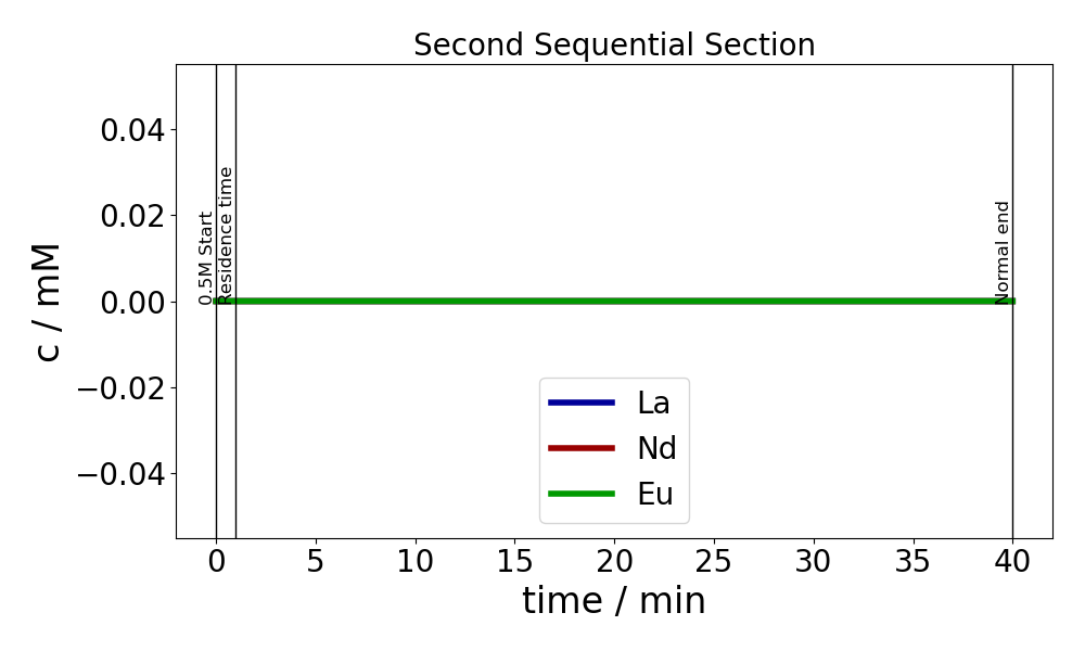
fig = plt.figure()
ax = fig.add_subplot()
ax.plot(time, c)
ax.set_xlabel(r'time / min')
ax.set_ylabel(r'c / mM')
ax.legend(component_system.names)
plt.title(f"Load [component]={load_comp[0]} mM, Col_length={column.length * 100:.2f} cm")
plt.axvline(column.calculate_interstitial_rt(initial_flowrate) / 60, color='k', lw=1)
plt.text(column.calculate_interstitial_rt(initial_flowrate) / 60, 0, "Residence time", rotation="vertical",
horizontalalignment="right", fontsize=12)
plt.axvline(process.section_times[5] / 60, color='k', lw=1)
plt.text(process.section_times[5] / 60, 0, "0.5M Start", rotation="vertical", horizontalalignment="right", fontsize=12)
plt.axvline(t / 60, color='k', lw=1)
plt.text(t / 60, 0, "Normal end", rotation="vertical", horizontalalignment="right", fontsize=12)
# Plot zoom settings:
# plt.xlim(0, 8)
# plt.ylim(0, 0.5e-10)
fig.tight_layout()
plt.savefig(os.path.join(WORKING_FOLDER, "ln-1_simple.png"))
# Calculate component yields
# NOTE: currently only accounts for the mobile phase.
# Construct flowrate array (fr): the flowrate at each time element.
idx_ifr = np.argwhere(time > process.events[5].time / 60)[0].item()
fr = np.ones([idx_ifr]) * initial_flowrate
fr = np.append(fr, np.ones([time.shape[0] - idx_ifr]) * elute_flowrate)
# How much goes in:
amt_in = {}
for component in range(3):
amt_in[component] = integrate.simpson(
y=np.multiply(model.root.output.solution.unit_001.solution_inlet_port_000[:, component], fr), x=time * 60) * 1E6
amt_in
# How much goes out:
amt_out = {}
for component in range(3):
amt_out[component] = integrate.simpson(
y=np.multiply(model.root.output.solution.unit_001.solution_outlet_port_000[:, component], fr),
x=time * 60) * 1e6
print(f"Recovery[{component_system[component].name}] = {100 * amt_out[component] / amt_in[component]:.2f}%")
# print("Column-bound component concentrations:")
# print(model.root.output.solution.unit_001.solution_solid[-1, :, :])