Multiple component adsorption

Hey everyone,

I am currently working on a master thesis where I look at competitive adsorption.
The literature for my topic has a lot of data for Freundlich constants, but in CADET only Multi component Langmuir is possible.
Is there a way to emulate something similar to a Mulit component Freundlich adsorption with the current CADET tools or this just not possible?

Thanks in advance

Hi Seemansgarn,
we’ve actually recently implemented the Freundlich isotherm. It’s not in the main branch yet but we will shortly make a new release. If you know how to compile CADET yourself, you can already check it out. Here is the corresponding PR: Feature/ldf isotherms by jazib-hassan-juelich · Pull Request #104 · modsim/CADET · GitHub
Best
Johannes

We have currently implemented the single component Freundlich model.

q = k_f c^n

However, it seems you are looking for a Freundlich-type multicomponent isotherm as described by Sheindorf et al. (1981).

q_i = k_f c_i \sum_{j=1}^{N_{c}}{a_{ij} c_j^{n-1}} with a_{ii}=1

We are currently looking into implement that one, too.

Do you have a timeline for the implementation of the Freundlich-type multicomponent isotherm?
It might influence my time frame/planning for the thesis.

It should be a matter of weeks. You might have to work with a development version until the new features are comprehensively tested and documented.

Adjacent question in this thread: would it be possible to add the Multicomponent Langmuir-Freundlich (Sips) isotherm into CADET? Thanks!

That is certainly possible. There are so many isotherm models, and we are implementing them upon request as our ressources allow. We can also teach users how to implemnt new isotherm models themselves. Do you have specific applications for the Sips model in mind?

I would be very interested in learning how to implement new isotherm models. How should we go about arranging this?

The particular application of Sips is for fitting of BT data that cannot be fit using multicomponent Langmuir (with GRM + surface diffusion) without making nonphysical assumptions. In short, the aggregate components have shallow uptake in the BT curve while the monomeric species do not. Fitting with MCL+GRM yields faster pore diffusion of the larger component if no assumptions are made. Both components should be excluded from the pores, based on iSEC measurements that we have performed. We are looking into performing some confocal experiments to evaluate if there is multilayer deposition or heterogeneous adsorption occurring, but do not have this data yet. I am wondering if Sips can be used to model this behavior where the BT front is curved when Dp is near-zero, since qmax is essentially variable.

@alters: How do the equations for the multi-component Sips isotherm look like?

@s.leweke I think it would look like this…

@alters Do you have literature references for that? The units of the adsorption and desorption constants seem odd. I assume you mean b_i instead of b,i. Technically, the model should be easy to implement as an extension of the existing multi-component Langmuir model.

We could reformulate using reference concentrations (which could be set to 1):

\frac{\partial q_i}{\partial t} = (k_{a,i})^{b_i} \left( \frac{c_{p,i}}{c_{ref,i} } \right)^{b_i} q_{max,i} \left( 1 - \sum_j \frac{q_j}{q_{max,j}} \right) - (k_{d,i})^{b_i} q_i

That’s certainly an option and should then be applied to q_i, too. But we should first clarify what the original equations are. It seems there are several variants with similar names.

I actually started to implement the SIPS model

\begin{align}\frac{\partial q_i}{\partial t} &= k_{ldf,i} \left( q_i^* - q_i \right) \\ q_i^* &= k_{f,i} c_{p,i} \left( \sum_j a_{ij} c_{p,j} \right)^{n_i - 1} \end{align}

from the Sheindorf paper using a linear-driving-force (LDF) approach.

However, I got stuck on linearizing the term

\left( \sum_j a_{ij} c_{p,j} \right)^{n_i - 1}

for small total concentration \sum_j a_{ij} c_{p,j}. My approach was similar to the single-component Freundlich isotherm.

  1. Define s_i := \sum_j a_{ij} c_{p,j}
  2. If s_i \leq T, where T is some threshold, we use a polynomial p(s_i) = b_1 s_i + b_2 s_i^2 instead of s_i^{n_i - 1}.
  3. I computed the coefficients b_1, b_2 based on the conditions p(T) = T^{n_i-1} and p'(T) = (n_i-1) T^{n_i-2} (i.e., continuity and continuity of derivative).

My problem is that I could not establish p(s) \geq 0 for s \in [0, T]. Do you think the approach is fundamentally flawed or do you have another idea?

Related: What is the range of the exponents n_i?

I found the following with the help of Mathematica.

Ansatz:

q_i^* = k_{f,i} c_{p,i} \left( \sum_j a_{i,j} c_{p,j} \right)^{n_i - 1}

p_{i,j}=b_{i,j,1} c_j+b_{i,j,2} c_j^2

Conditions:

p_i(c_j=T)=q_i^*(c_j=T)

\frac{\partial p_i}{\partial c_j}(c_j=T)=\frac{\partial q_i^*}{\partial c_j}(c_j=T)

Coefficients for i=j:

b_{i,i,1}= k_f \left((2-n_i) a_{i,i} T + \sum_{k \neq i}{a_{i,k} c_k}\right) \left(a_{i,i} T + \sum_{k \neq i}{a_{i,k} c_k}\right)^{n_i-2}

b_{i,i,2}=k_f (n_i-1) a_{i,i} \left(a_{i,i} T+ \sum_{k \neq i}{a_{i,k} c_k}\right)^{n_i-2}

Coefficients for i \neq j:

b_{i,j,1}=k_f\frac{c_i}{T} \left((3-n_i) a_{i,j} T+2\sum_{k \neq i}{a_{i,k} c_k}\right) \left(a_{i,j} T+\sum_{k \neq i}{a_{i,k} c_k}\right)^{n_i-2}

b_{i,j,2}= k_f\frac{c_i}{T^2} \left((n_i-2) a_{i,j} T+\sum_{k \neq i}{a_{i,k} c_k}\right) \left(a_{i,j} T+ \sum_{k \neq i}{a_{i,k} c_k}\right)^{n_i-2}

In case c_j<T for more than one index j, I would propose a weighted sum of the corresponding approximations:

p_i^*=\frac{\sum_j{w_j p_{i,j}}}{\sum_j{w_j}}

with weights:

w_j=\max{(0,\frac{T-c_j}{T})}

Please double check for flaws and typos.

Thanks, @lieres. You propose to interpolate the full equilibrium concentration q_i^* instead of the nonlinear part.

Now, numerical problems only emerge if \sum_j a_{ij} c_{p,j} \approx 0. It’s totally fine for some of the c_{p,j} to be small as long as this weighted sum is positive. So what is the reason for distinguishing here?

Another idea: Because of the form of the equation, I think that adding a small constant (say \tau \approx 10^{-10}) would also work:

q_i^* = k_{f,i} c_{p,i} \left( \sum_j a_{ij} c_{p,j} + \tau \right)^{n_i - 1}

Because the term in the parentheses is multiplied by c_{p, i}, it will still hold that q_i^* = 0 for c_{p,i} = 0.

What do you think about it? Of course, this hinges on the assumption that a_{i,j} \geq 0.

@Seemansgarn: Can you clarify the ranges / constraints of a_{ij}, n_i ? Are they non-negative, positive, etc.?

To my understanding the numerical probelms are caused by the derivative of the nonlinear equation approaching \infty for small concetrations. This is why I have linearized the whole equation around the origin. The weighted sum is neccessary to achieve a smooth transition between cases where one or another component concentration crosses the threshold T.

Your idea with adding \tau is obviously much simpler and certainly worth investigating.

My apologies for the late reply. It should have been b_i not b,i. I just obtained this expression using MCL as a basis and assembling it in the kinetic form accordingly. I haven’t found publications using this model in the kinetic form, thus far, but I will take a closer look.

Thank you guys for working on this! It is quite interesting to see the mathematical development in action!

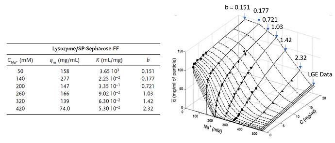
The way I have used this model in its equilibrium form (fitting batch data) was with kA and qMax having the same constraints they would in Langmuir (both nonzero and strictly positive). I have used the b parameter with the same constraints. Of course for b = 1 it becomes the Langmuir isotherm. Adjusting the b values should allow for some flexibility in the binding affinity and, accordingly, the shape of the initial and transition regions of the isotherm (at equilibrium). Here is a figure from Creasy et al. 2015 in Biotech Journal discussing their construction of an empirical isotherm (EI). You can see the impact of the b values clearly when you arrive at an S-shaped isotherm for b > 1. For b < 1 the uptake may be slower, depending on the concentrations and the value of K.

I am not completely sure how this model would translate to simulations of breakthrough curves, which is what we want to test this on. The hope is that it allows us to have some flexibility in the shape of the uptake without having to change intraparticle diffusion rates.

I am not sure yet about the particular ranges of a_ij and n_i yet but I will check back in later to see how these are affected by the b values in the transition to the formulation using LDF. I would think that they should also be positive and nonzero, however I could of course be incorrect. Nonetheless, I hope this is helpful.

Hi Sam,

Just to check in briefly - what is the progress on implementing the langmuir-freundlich in CADET? We would be more than happy to help test the model.

Thanks a lot for working on this, we very much appreciate it!