negative elution with Langmuir MPM

[rosario.cervellere]

Expected behavior.

Fit Langmuir MPM parameters (offline) to match desired pH dependence. Use fit params to simulate bind, wash, and elute.

Actual behavior

With certain combinations of MPM params (Ka, gamma, beta) , no binding occurs and during elution the outlet concentration dives negative.

How to produce bug (including a minimal reproducible example)

import pandas as pd
import numpy as np
#from numpy import trapezoid
import matplotlib.pyplot as plt
# import cadet packages
from CADETProcess.processModel import ComponentSystem
from CADETProcess.processModel import LangmuirLDF
from CADETProcess.processModel import MobilePhaseModulator
from CADETProcess.processModel import Inlet, LumpedRateModelWithoutPores, Outlet
from CADETProcess.processModel import TubularReactor, Cstr
from CADETProcess.processModel import FlowSheet
from CADETProcess.processModel import Process
from CADETProcess.reference import ReferenceIO
from CADETProcess.comparison import Comparator
from CADETProcess.optimization import OptimizationProblem
from CADETProcess.optimization import U_NSGA3
# --------------------------
# setup experiment
# --------------------------
mLmin_to_m3s = 60*1e6 # conversion
exp_flow = 8. # MV/min (mL/min)
Q = exp_flow/(mLmin_to_m3s) # convert to m^3/s
size_kDa = 150 # protein size
Qmax = 80 # mg/mL = g/L
Qmax_mMol = Qmax/size_kDa
# -------------------------------------
# load and wash and elute volumes and pH
# -------------------------------------
loadVol = 60.1 #42.3 #43.0 #60.1 # mL
washVol = 35.35 #33.9 #25.0 #34.8 # mL
eluteVol = 12. # mL
protein_c = 3.5 #3.7 #3.6 #3.5 # g/L
pH_bind = 7.5
pH_elute = 3.8
pH_b_H = 10**(-pH_bind)
pH_e_H = 10**(-pH_elute)

#print(pH_range)
#print(pH_b_H, 'bind')
#print(pH_e_H,'elute')
# --------------------------------------
# calculating timepoints for experiment
# --------------------------------------
total_vol = loadVol + washVol + eluteVol # mL
exp_time = total_vol/exp_flow*60 # seconds
sample_vol = loadVol
load_time = loadVol/(exp_flow/60.)
wash_time = washVol/(exp_flow/60.)
elute_time = eluteVol/(exp_flow/60.)
# ---------------------------------------------------
# CSTR and tubing lenght parameters from system fit
# ---------------------------------------------------
sys_CSTR_vol = 0.116e-6 # m^3
sys_tubing_len = 3.086 # m
# --------------------------------
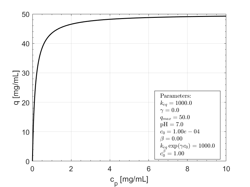
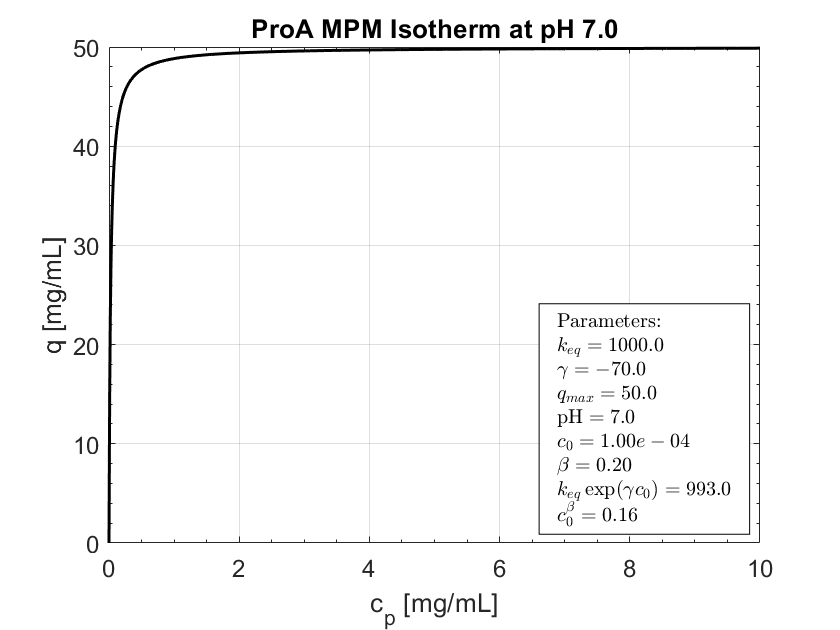
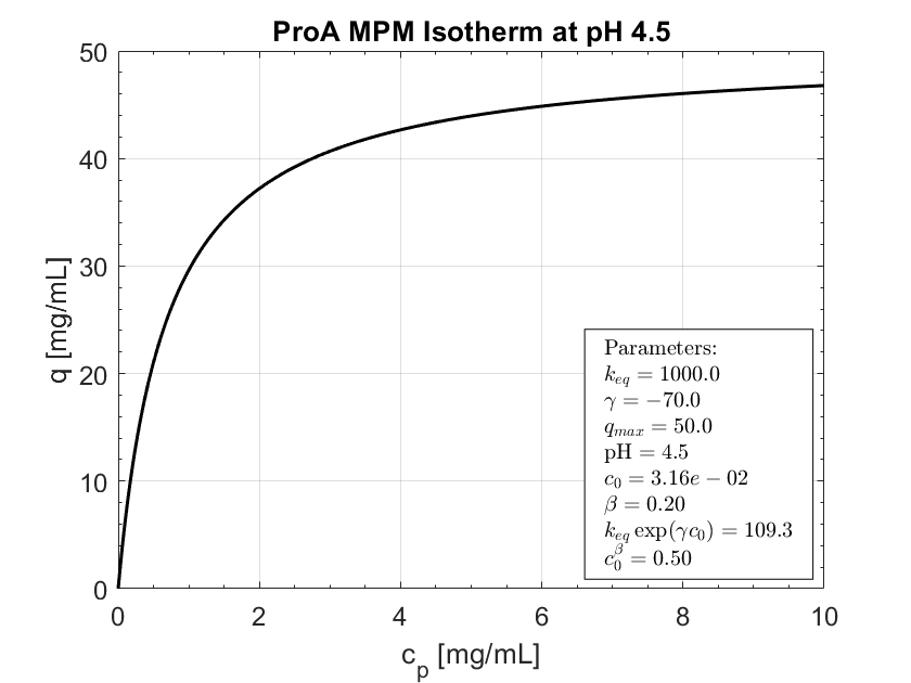
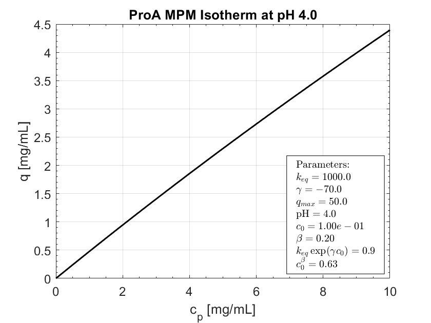
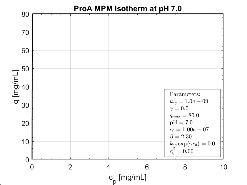
# MPM fitting coefficients, keq = Ka * \frac{e^{\gamma*[H+]}}{[H+]^\beta}
# --------------------------------
# !!!!!! varying combinations of these parameters introduces numerical artifacts, 
# no bidning, negative elution, etc.... how do I avoid this?
Ka = 1.0e-9 # similar issue with beta
gamma = 0
beta = 2.3 # 2.29 works, not 2.3
# ---------------------------
# create component system
# ---------------------------
component_system = ComponentSystem(['pH','protein'])
# -------------------------
# binding model 
# -------------------------
binding_model = MobilePhaseModulator(component_system, name='MPM')
# setup system to use keq = a * np.exp[H+]/[H+]^\beta
binding_model.is_kinetic = False
binding_model.desorption_rate = [0.,1.]
binding_model.capacity = [0,Qmax_mMol]
binding_model.ion_exchange_characteristic = [0, beta] 
binding_model.hydrophobicity = [0, gamma] 
binding_model.adsorption_rate =[0,Ka]
binding_model.desorption_rate = [0,1]
binding_model.bound_states=[0,1]
binding_model.check_required_parameters()
# -------------------------
# setup BWE buffers
# -------------------------
# feed (mAb05)
feed = Inlet(component_system, name='feed')
feed.c = [pH_b_H,protein_c/size_kDa]
# wash (washout buffer)
wash = Inlet(component_system, name='wash')
wash.c = [pH_b_H,0]
# elute (elution buffer)
elute = Inlet(component_system, name='elute')
elute.c = [pH_e_H,0]
# ----------------------
# device 
# ----------------------
device = LumpedRateModelWithoutPores(component_system, name='device')
device.length = 0.0193*8/100 # m 
device.diameter = 2.85/100 # m 
device.total_porosity = 0.55 # estimate
device.axial_dispersion = 1e-12 # near zero
device.binding_model = binding_model
device.discretization.ncol = 20 # i've gone up to 1000, still an issu
device.c = [pH_b_H,0]
#device.discretization.use_analytic_jacobian = False
# ----------------------
# feed tubing
# ----------------------
load_tubing = TubularReactor(component_system, name='load_tubing')
load_tubing.c = [pH_b_H,0]
load_tubing.length = sys_tubing_len # m #270/100
load_tubing.diameter = 0.75/1000
load_tubing.axial_dispersion = 1e-12
load_tubing.discretization.ncol=20
# ----------------------
# outlet
# ----------------------
outlet = Outlet(component_system, name='outlet')
outlet.solution_recorder.write_solution_bulk = True
# -----------------------
# inlet CSTR
# -----------------------
cstr_vol = 0.18e-6 # m^3
inlet_mixer = Cstr(component_system, name='inlet_mixer')
inlet_mixer.c = [pH_b_H,0]
inlet_mixer.init_liquid_volume = 1.0*cstr_vol # m^3
inlet_mixer.check_required_parameters()
#inlet_mixer.solution_recorder.write_solution_bulk=True
# ------------------------
# outlet CSTR
# ------------------------
outlet_mixer = Cstr(component_system, name='outlet_mixer')
outlet_mixer.c = [pH_b_H,0]
outlet_mixer.init_liquid_volume = 7.0*cstr_vol # m^3
outlet_mixer.check_required_parameters()
#outlet_mixer.solution_recorder.write_solution_bulk=True
# ------------------------
# detector CSTR
# ------------------------
detector_mixer = Cstr(component_system, name='detector_mixer')
detector_mixer.c = [pH_b_H,0]
detector_mixer.init_liquid_volume = 0.2e-6 # m^3 (0.2 mL detector volume)
detector_mixer.check_required_parameters()
# ------------------------
# system CSTR
# ------------------------
system_mixer = Cstr(component_system, name='system_mixer')
system_mixer.c = [pH_b_H,0]
system_mixer.init_liquid_volume = sys_CSTR_vol # m^3
system_mixer.check_required_parameters()

# ------------------------------------------------
# now we create the Flow Sheet
# ------------------------------------------------
flow_sheet = FlowSheet(component_system)
flow_sheet.add_unit(feed)
flow_sheet.add_unit(wash)
flow_sheet.add_unit(elute)
flow_sheet.add_unit(load_tubing)
flow_sheet.add_unit(device)
flow_sheet.add_unit(outlet)
flow_sheet.add_unit(inlet_mixer)
flow_sheet.add_unit(outlet_mixer)
flow_sheet.add_unit(detector_mixer)
flow_sheet.add_unit(system_mixer)
# connect components
flow_sheet.add_connection(feed, system_mixer)
flow_sheet.add_connection(wash, system_mixer)
flow_sheet.add_connection(elute, system_mixer)
flow_sheet.add_connection(system_mixer, load_tubing)
flow_sheet.add_connection(load_tubing, inlet_mixer)
flow_sheet.add_connection(inlet_mixer,device)
flow_sheet.add_connection(device, outlet_mixer)
flow_sheet.add_connection(outlet_mixer, detector_mixer)
flow_sheet.add_connection(detector_mixer, outlet)
# --------------------------------------------------------------
# now we create the process, i.e., turning feed on, swap to wash buffer, same flow rate
# --------------------------------------------------------------
process = Process(flow_sheet, 'breakthrough')
process.add_event('feed_on','flow_sheet.feed.flow_rate',Q,time=0)
process.add_event('feed_off','flow_sheet.feed.flow_rate',0,time=load_time)
# wash
process.add_event('wash_on','flow_sheet.wash.flow_rate',Q,time=load_time)
process.add_event('wash_off','flow_sheet.wash.flow_rate',0,time=load_time+wash_time)
# elute
process.add_event('elute_on','flow_sheet.elute.flow_rate',Q,time=load_time + wash_time)
process.add_event('elute_off','flow_sheet.elute.flow_rate',0,time=exp_time)
# cycle time
process.cycle_time = exp_time # seconds
#process.n_cycles = 1
# -----------------------------
# simluate the process
# -----------------------------
if __name__ == '__main__':
    from CADETProcess.simulator import Cadet
    process_simulator = Cadet()
    process_simulator.time_resolution = 0.1
    simulation_results = process_simulator.simulate(process)
# ------------------------------
# save x- and y- axis information
# ------------------------------
x_axis_sim_init = simulation_results.solution.outlet.outlet.time
x_axis_sim_min = x_axis_sim_init/60.
y_axis_sim_init = simulation_results.solution.outlet.outlet.solution
y_axis_sim_init = y_axis_sim_init[:,1]
# ----------------------------
# plot simulation
# ----------------------------
plt.plot(x_axis_sim_min*exp_flow,y_axis_sim_init*size_kDa,'-b',label='BWE simulation')
plt.ylabel('g/L')
plt.xlabel('mL')
plt.legend()

File produced by conda env export > environment.yml

environment.yml (7.56 KB)

[rosario.cervellere]

Is there a way to decrease the time stepping to help with stability? Reading through some of the documentation it isn’t quite clear how to control some of these numerical instabilities when they arise

[rosario.cervellere]

I believe I found the issue. When Keq > 1e8 the simulation does not run successfully. Why this is the case? I’m unsure… I’m assuming it has to do with floating point operations.

Is there a way I can make a conditional statement for the simulation in CADET-Process?

Something like:

If Keq > 1e8 then Keq == 1e8

[alters]

I was quite curious about how this model would work for proA or other affinity systems with low pH elution. A really good way to understand how the isotherm model works is to calculate the equilibrium solid phase concentration q as a function of the liquid phase concentrations – c_p (protein) and c_0 (H+ ion). In this way, we can isolate the isotherm from the transport model and analyze the isotherm properties as a function of model parameters. In other words, we can play with the model parameters and directly assess what the impact will be.

First, let’s derive the single component MPM isotherm formalism in equilibrium form:

Start with single-component kinetic form

\frac{\mathrm{d} q}{\mathrm{~d} t}=k_{a} \exp({\gamma c_{0})} c_{p} q_{\max}\left(1-\frac{q}{q_{max}}\right)-k_{d} c_{0}^{\beta} q

At equilibrium, \frac{\mathrm{d} q}{\mathrm{~d} t}=0, therefore

0=k_{a} \exp\left({\gamma c_{0}}\right) c_{p} q_{\max}\left(1-\frac{q}{q_{max}}\right)-k_{d} c_{0}^{\beta} q

As a simplification, we use k_{eq} = k_a/k_d – dividing by k_d gives us

0=k_{eq} \exp\left({\gamma c_{0}}\right) c_{p} q_{\max}\left(1-\frac{q}{q_{max}}\right)-c_{0}^{\beta} q

Algebraic manipulation gives us the final equation

q = \frac{k_{eq}\exp\left({\gamma c_{0}}\right)q_{max}c_p}{k_{eq}\exp\left({\gamma c_{0}}\right)c_p+c_0^\beta}

c_0 is the modulator concentration – in this case it is the H+ concentration in mol/m^3 or mM. So, pH 7 would correspond to c_0 = 10^{-4}. We also need to make sure that q and q_{max} are in units of mmol protein / L solid phase. For example, a q_{max} of 50 g/L would be converted by dividing by molecular weight (kDa) and dividing by (1-\varepsilon_t), where \varepsilon_t is the total porosity (set to 0.9 in this example). After our calculations of q, we can convert all units back to their original state to help with interpretation.

Example isotherm:

Analysis of isotherm shapes allows us to define some appropriate (example) ranges of parameters k_{eq}, q_{max}, \gamma, and \beta.

q_{max} \in \left[0,100\right], a realistic range (in \mathrm{g/L})

k_{eq} \in \left[0,1000\right], a realistic range (in \mathrm{L/g})

\gamma \in \left[-100,0\right], to ensure that q decreases exponentially with increasing c_0. This parameter needs to be negative and cannot be neglected. Units are \mathrm{mM^{-1}}.

\beta\ \in [-0.5,0.5], this is a weird one – as \beta increases, q rapidly approaches
q_{max}. Conversely, as \beta decreases, q rapidly approaches 0. I would treat this as a fitting parameter or set it to zero to ignore it (this should be acceptable, I think).

Applying some reasonable estimates give us the isotherm, first at pH 7.0 – should expect favorable isotherm.

Then at pH 4.5 – should expect weaker affinity as compared to pH 7.0, but still maintaining capacity.

Then at pH 4.0 – should expect almost no more binding.

These isotherms follow the expected trends in proA. You can also see how critical \gamma is in the model since it entirely controls the pH dependence. \beta can be finely tuned in a narrow range – I suppose it might help with capturing subtleties, but definitely be careful with it.

You should be able to use these ranges for your simulations in CADET, just make sure to keep all the units consistent. For example, if you used c_0 in M you’d need to change your range for \gamma.

Hope this helps!

[alters]

Also, to your previous comments: I think you are getting strange behavior because the parameters you specified lead to extremely high affinities which also can break the solver. If you stick to the ranges we derived, I don’t think you should have any issues with stability.

BTW, this is the isotherm I got with the inputs in your original post. You can see that it is unrealistically square, which breaks the solver. This is why it is so important to isolate the isotherm
model and study the model parameter relationships! Otherwise, it is quite difficult to understand what reasonable parameter values would even be.