I was quite curious about how this model would work for proA or other affinity systems with low pH elution. A really good way to understand how the isotherm model works is to calculate the equilibrium solid phase concentration q as a function of the liquid phase concentrations – c_p (protein) and c_0 (H+ ion). In this way, we can isolate the isotherm from the transport model and analyze the isotherm properties as a function of model parameters. In other words, we can play with the model parameters and directly assess what the impact will be.
First, let’s derive the single component MPM isotherm formalism in equilibrium form:
Start with single-component kinetic form
\frac{\mathrm{d} q}{\mathrm{~d} t}=k_{a} \exp({\gamma c_{0})} c_{p} q_{\max}\left(1-\frac{q}{q_{max}}\right)-k_{d} c_{0}^{\beta} q
At equilibrium, \frac{\mathrm{d} q}{\mathrm{~d} t}=0, therefore
0=k_{a} \exp\left({\gamma c_{0}}\right) c_{p} q_{\max}\left(1-\frac{q}{q_{max}}\right)-k_{d} c_{0}^{\beta} q
As a simplification, we use k_{eq} = k_a/k_d – dividing by k_d gives us
0=k_{eq} \exp\left({\gamma c_{0}}\right) c_{p} q_{\max}\left(1-\frac{q}{q_{max}}\right)-c_{0}^{\beta} q
Algebraic manipulation gives us the final equation
q = \frac{k_{eq}\exp\left({\gamma c_{0}}\right)q_{max}c_p}{k_{eq}\exp\left({\gamma c_{0}}\right)c_p+c_0^\beta}
c_0 is the modulator concentration – in this case it is the H+ concentration in mol/m^3 or mM. So, pH 7 would correspond to c_0 = 10^{-4}. We also need to make sure that q and q_{max} are in units of mmol protein / L solid phase. For example, a q_{max} of 50 g/L would be converted by dividing by molecular weight (kDa) and dividing by (1-\varepsilon_t), where \varepsilon_t is the total porosity (set to 0.9 in this example). After our calculations of q, we can convert all units back to their original state to help with interpretation.
Example isotherm:
Analysis of isotherm shapes allows us to define some appropriate (example) ranges of parameters k_{eq}, q_{max}, \gamma, and \beta.
q_{max} \in \left[0,100\right], a realistic range (in \mathrm{g/L})
k_{eq} \in \left[0,1000\right], a realistic range (in \mathrm{L/g})
\gamma \in \left[-100,0\right], to ensure that q decreases exponentially with increasing c_0. This parameter needs to be negative and cannot be neglected. Units are \mathrm{mM^{-1}}.
\beta\ \in [-0.5,0.5], this is a weird one – as \beta increases, q rapidly approaches
q_{max}. Conversely, as \beta decreases, q rapidly approaches 0. I would treat this as a fitting parameter or set it to zero to ignore it (this should be acceptable, I think).
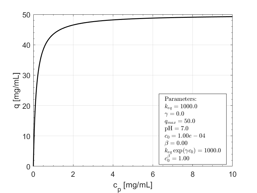
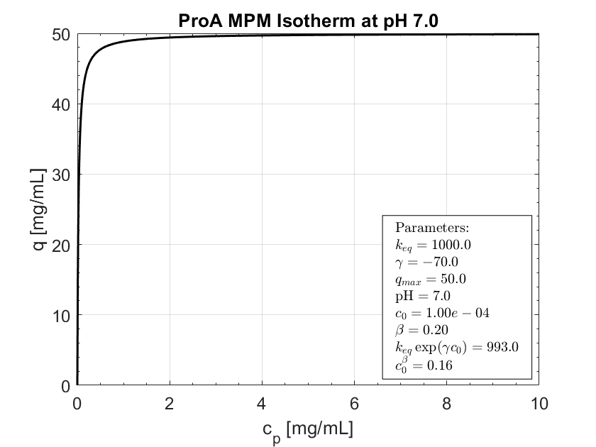
Applying some reasonable estimates give us the isotherm, first at pH 7.0 – should expect favorable isotherm.
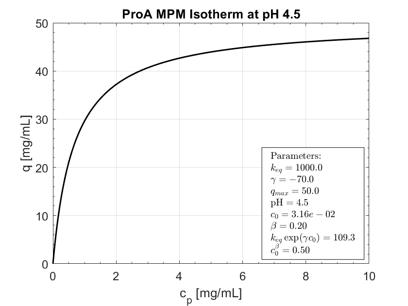
Then at pH 4.5 – should expect weaker affinity as compared to pH 7.0, but still maintaining capacity.
Then at pH 4.0 – should expect almost no more binding.
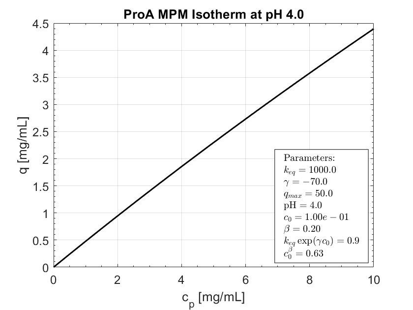
These isotherms follow the expected trends in proA. You can also see how critical \gamma is in the model since it entirely controls the pH dependence. \beta can be finely tuned in a narrow range – I suppose it might help with capturing subtleties, but definitely be careful with it.
You should be able to use these ranges for your simulations in CADET, just make sure to keep all the units consistent. For example, if you used c_0 in M you’d need to change your range for \gamma.
Hope this helps!