Question on hyperthreading in CADET

[alters]

Hi all,

I had some general questions involving how CADET employs hyperthreading when performing simulations.

When specifying number of threads in the CADET simulation framework (sim.nThreads), how are the multiple threads used in a single CADET simulation? I was under the impression that the solution in its time and spatial elements was sequential and not parallelizable, however I could be totally off-base here.

Which scenario (out of the below two) would we expect to be more efficient for parameter fitting (assuming the algorithm itself is parallelizable e.g. genetic algorithm)?

1. Running 10 simulations in parallel with each simulation containing 1 thread
2. Running only 1 simulation at a time with each simulation containing 10 threads

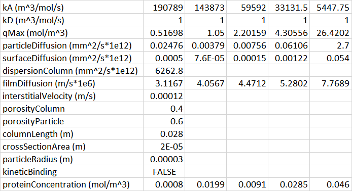
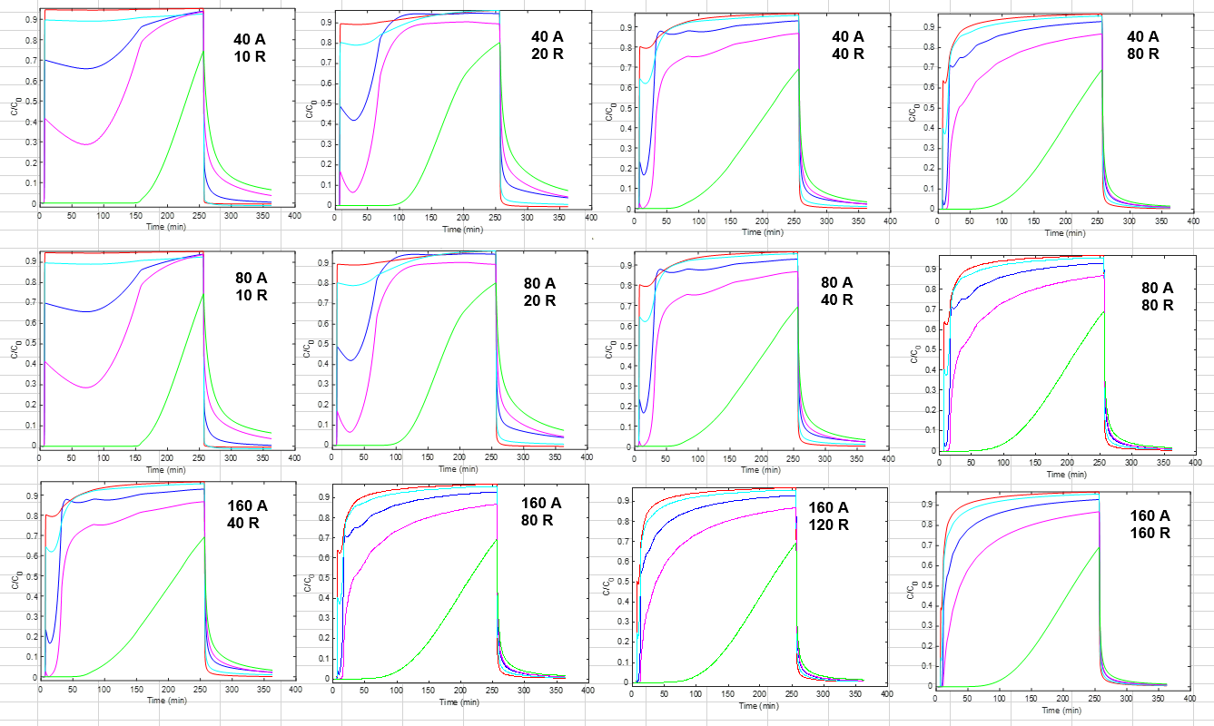
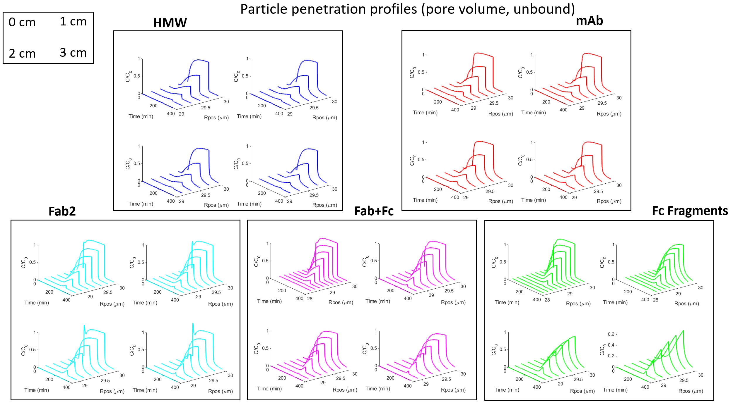
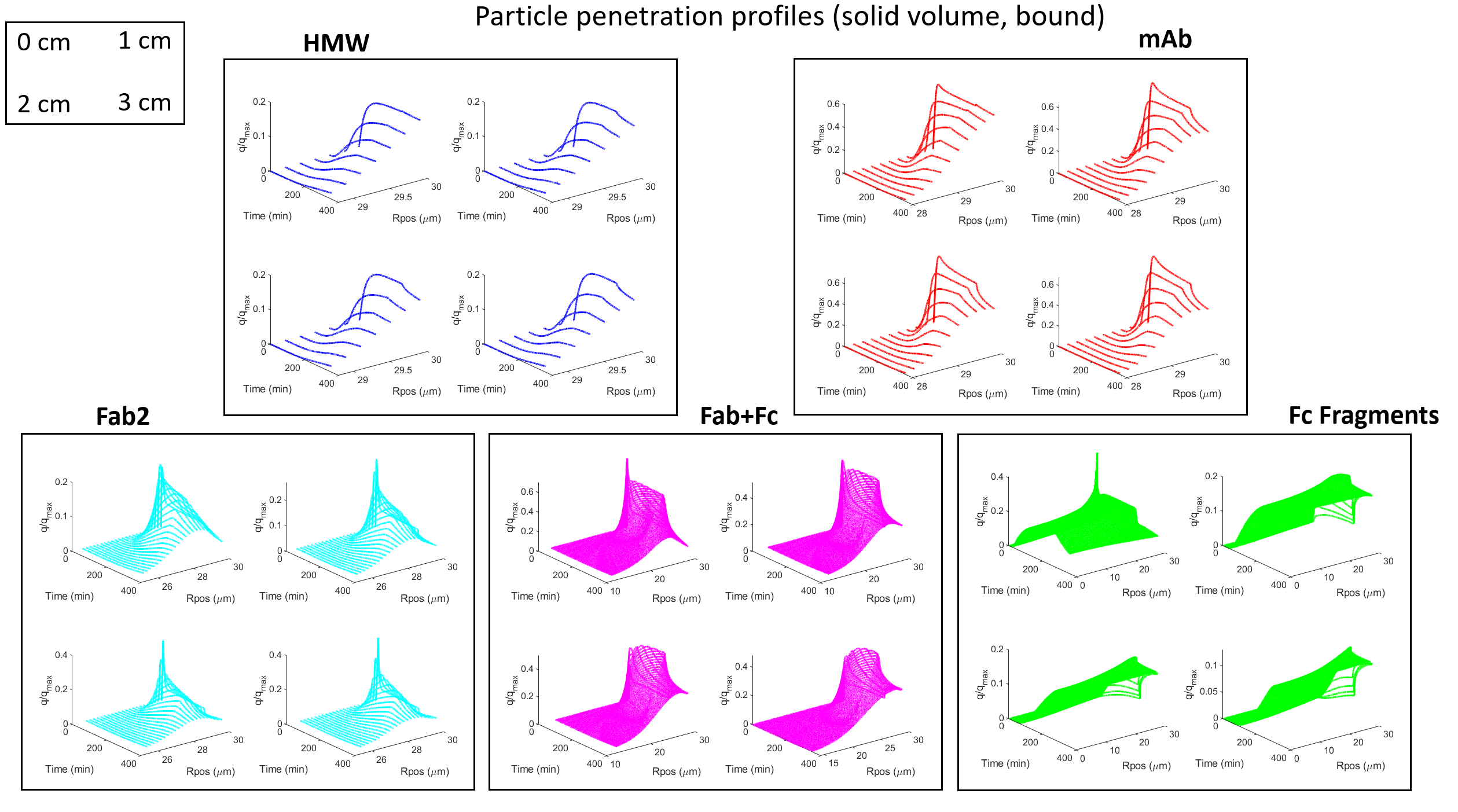
For some context: I am fitting a set of BT curves (single salt/pH, multiple residence times) in CADET MATLAB using the GRM and multicomponent Langmuir isotherm with five protein components. There are many parameters to be fitted here and the simulations are quite slow since I am using a large number of discretizations (150 axial, 100 radial) because there are anomalous fronts in the BT curves that appear otherwise. I have been experimenting with different optimization methods and found that MATLAB surrogateopt (surrogate optimization) is a good option for this problem. I have also spent a considerable amount of time to narrow down the search space of the parameters (kA, qMax, particleDiffusion). The resin in question here has extremely small pores and very strong binding.

Thanks for the help!
Scott

[s.leweke]

Hey Scott,

TL;DR:

@alters

Which scenario (out of the below two) would we expect to be more efficient for parameter fitting (assuming the algorithm itself is parallelizable e.g. genetic algorithm)?

1. Running 10 simulations in parallel with each simulation containing 1 thread
2. Running only 1 simulation at a time with each simulation containing 10 threads

Choose option 1, or a hybrid (say, 5 simulations in parallel each using 2 threads or 3 sims each using 3 threads).

Long version
Parallelization is a difficult subject. A simulation has essentially two “directions” to parallelize: Space and time. Time stepping is inherently serial (you need the current state in order to do a step into the future). This is why very sophisticated methods are required for parallelization in time. These methods do exist, but because they are so complex, we have not implemented any of them in CADET. As far as I know, the return on investment is rather small compared to parallelization in space. So you turn to parallelization in time only if you cannot achieve substantial gains by parallelization in space (kind of a last resort).

This leaves parallelization in space. We use a nested approach here: On the first level, we can parallelize the full system of unit operations (i.e., each unit operation can be solved in parallel). This is useful if you are dealing with systems composed of multiple columns (e.g., simulated moving bed).

Second, we can parallelize the solution on the unit operation level (provided the model is complex enough). This is support for lumped rate model with pores (LRMP) and above, including the general rate model. The idea is to solve the interstitial volume and all the particles in parallel. For the general rate model, there are NCOL + 1 tasks created that are completed in parallel. One task for each particle (150 reference particles in your case, each having 100 radial shells) and one task for the interstitial volume (comprised of 150 axial cells).

We have conducted some benchmarks that show a moderate scaling for up to 4 (maybe 6) threads with diminishing gains beyond this. For the parallelization to show effect, a beefy problem is required – which you have. Still, the scaling is far from optimal.

If you want to read up on this, I refer you to my thesis (shameless plug, also a little technical). In particular, Sec. 3.8 on nested parallelization and Sec. 5.1-5.2 on benchmarking.

In order to reduce the amount of cells required, we are also working on another discretization method (discontinuous Galerkin). This method has the potential of substantially reducing the number of cells due to higher order discretization. It’s not ready yet, though.

@alters

I am using a large number of discretizations (150 axial, 100 radial) because there are anomalous fronts in the BT curves that appear otherwise.

Do you mind showing some plots of these strange fronts? Do you use surface diffusion?

[alters]

Hi Sam,

Thanks for your quick response! The explanation on how the parallelization in space makes a lot of sense. It is helpful to have your thesis as well, so thanks for sharing this. I was wondering what the methods used for parallelization in time are called, just out of curiosity. Also, can you explain what the difference is between discontinuous Galerkin discretization method compared to the method that is currently implemented in CADET? I am not entirely sure which method is used currently.

I am including some figures here of the BT curve simulations run at different sets of axial and radial discretization. The parameters for the simulations are included below as well. I use surface diffusion as a constant value of pore diffusion / 50, which is reasonable, I think, for very strong binding conditions.

Multicomponent Langmuir with GRM

See figures below. Each color is one protein component. For reference, this process is expected to be pore diffusion controlled (separation mechanism based on size partitioning) with some multicomponent effects. You can see below that there are anomalies in the front of the BT curve that aren’t resolved unless very high numbers of discretization are selected. The tail of the BT curve is affected as well. Radial nodes seem to be particularly important and need to be above 100. I am not entirely sure why these anomalies are developing (numerical dispersion, sure) but I think it has something to do with the sharp breakthroughs that occur since some of the components have near-zero diffusion rates and breakthrough almost immediately, maybe causing discontinuities in the pore concentration rate terms…

What are your thoughts?

Thanks,
Scott

[s.leweke]

@alters

I was wondering what the methods used for parallelization in time are called, just out of curiosity.

There are several methods: Parareal, space-time multigrid,parallel Runge-Kutta, to name a few. Here are some more.

@alters

Also, can you explain what the difference is between discontinuous Galerkin discretization method compared to the method that is currently implemented in CADET

CADET uses the finite volume (FV) method in combination with a WENO scheme for computing the numerical fluxes. This results in a scheme that is second order convergent. In the finite volume method, the computational domain is divided into cells. In each cell, we approximate the average of the solution by mass balances (i.e., tracking the influx, outflux and reaction). The cell average of the solution (i.e., the numerical solution) is actually a second-order accurate approximation of the true solution at the center of the cell.

Discontinuous Galerkin (DG) is more sophisticated and provides higher-order convergence. That is, we can have a much higher accuracy with the same number of unknowns; or, the same accuracy with a much lower number of unknowns. Thus, we can get quite some speedup compared to the low-order finite volume scheme we are using now. DG also divides the domain into cells, but uses a linear, quadratic, or cubic (or even higher order) approximation of the solution within each cell instead of the solution’s average. Therefore, you get a much higher resolution with the same number of cells compared to FV.

There certainly is a lot of stiffness in your problem as your parameters span multiple orders of magnitude. The pore diffusion coefficients span 2 orders of magnitude, the surface diffusion coefficients three. With these parameters, it could be the case that this level of resolution (i.e., number of particle shells) is simply required.

Doing a mesh-independence study, like you have done here, is good practice. I don’t think that with these parameters you can get around with fewer cells. The story would be different with DG and its higher-order approximation capabilities. Here, you should be able to ramp up the order and decrease the number of cells.

This could actually be a very interesting test case for us while developing the DG method. Thanks for providing the parameters!

[alters]

Thanks for your response, Sam! This is very interesting and is quite helpful for our understanding of the software as well as the general mathematical methods that are employed. When do you think the DG method will be integrated into CADET? It sounds quite promising.

With respect to the solution stiffness could you please elaborate on why the difference in orders of magnitude for the diffusion parameters will have an impact?

I am glad the parameters are helpful for the development of DG in CADET. Please let me know if I missed any in the set and I can provide them. The crossSectionArea should have been in m^2 units, that was an error.

Scott

[lieres]

I don’t want to promise anything, but if you are lucky we can provide you with a development version of the DG method in a couple of weeks. You could then take part in testing the code.

[alters]

That is excellent news! I would be happy to help test the code, seeing as I am running CADET daily for this portion of my thesis, and hopefully be able to assist you guys in some way.

Thanks,
Scott

[s.leweke]

Another idea to maybe get a feeling of what’s going on: Plot the solution in the interstitial and particle volume. For this, we need to enable output of the data first. As indicated in the docs, you need to set /input/return/unit_XYZ/WRITE_SOLUTION_BULK, /input/return/unit_XYZ/WRITE_SOLUTION_PARTICLE, and /input/return/unit_XYZ/WRITE_SOLUTION_SOLID to 1. Then, running a simulation will produce the output arrays:

• /output/solution/unit_XYZ/SOLUTION_BULK in nTime x nAxial x nComp format
• /output/solution/unit_XYZ/SOLUTION_PARTICLE in nTime x nAxial x nParticleShell x nComp format
• /output/solution/unit_XYZ/SOLUTION_SOLID in nTime x nAxial x nParticleShell x nComp format

For the formats above, I have assumed that you have a single particle type and use the 1D general rate model with one bound state per component.

[alters]

Hi Sam,

I have included some snapshots of the profiles in the pore volume for both the unadsorbed (top five figures) and adsorbed phase (bottom five figures). The four figures in each section are radial profiles w.r.t. time taken at specified distances in the column (0, 1, 2, 3 cm for a 3 cm column). While profiles in the unbound state (result.solution.particle) show that the penetration is minimal for all components, the bound state profiles (result.solution.solid) show that there is a significant difference. This seems reasonable due to the isotherm being extremely favorable.

Since the penetration into the particle is so minimal, it may be that many radial nodes are needed for the size of the discretized shell to match the length scale of the diffusion.

What do you think?