Here is a working example
from cadet import Cadet
import numpy as np
import matplotlib.pyplot as plt
Cadet.cadet_path = ## add your path
n_sites = 1
Q = 2.5 / (6e7) # volumetric flow rate m^3/s
## kd, eta, pka
kd = np.array([1,])
keq = np.array([10,])
qmax = np.array([62,])
## set up
c_feed = 8.0 / 150 # mol/m^3 (devide mg/mL by 150)
simulation_end_time1 = 1200
column_length = 0.05 # m
column_volume = 5.025e-6 # m^3
column_porosity = 0.37
particle_porosity = 0.97
protein_MW = 150
total_porosity = column_porosity + (1.0-column_porosity)*particle_porosity
#### part I simulation
def create_model(qmax, keq, Dp):
model = Cadet()
model.root.input.model.nunits = 3
model.root.input.model.unit_000.unit_type = 'INLET'
model.root.input.model.unit_000.ncomp = 1
model.root.input.model.unit_000.inlet_type = 'PIECEWISE_CUBIC_POLY'
model.root.input.model.unit_001.unit_type = 'GENERAL_RATE_MODEL'
model.root.input.model.unit_001.ncomp = 1
## Geometry
model.root.input.model.unit_001.col_length = column_length # m
model.root.input.model.unit_001.cross_section_area = column_volume/column_length # m^2
model.root.input.model.unit_001.col_porosity = column_porosity # 1
model.root.input.model.unit_001.par_porosity = particle_porosity # 1
model.root.input.model.unit_001.par_radius = 0.045e-3 # m
## Transport
model.root.input.model.unit_001.col_dispersion = 2.061e-8 # m^2/s
model.root.input.model.unit_001.film_diffusion = [1.18e-5] # m/s
model.root.input.model.unit_001.par_diffusion = [Dp,] # m^2/s [0.55e-11]
model.root.input.model.unit_001.par_surfdiffusion = n_sites * [0.0, ]
model.root.input.model.unit_001.adsorption_model = 'MULTI_COMPONENT_LANGMUIR'
model.root.input.model.unit_001.adsorption.is_kinetic = 0
model.root.input.model.unit_001.adsorption.mcl_ka = protein_MW*(1.0-total_porosity) * keq ## m^3 solid phase / mol protein / s ml/mg=m^3/kg 1 kda = 1 kg/mol
model.root.input.model.unit_001.adsorption.mcl_kd = kd ## s^-1
model.root.input.model.unit_001.adsorption.mcl_qmax = qmax/protein_MW/(1.0-total_porosity) ## mol/m^3 solid phase mg/ml=kg/m^3 / 150 kg/mol = 1/150 mol/m^3
model.root.input.model.unit_001.init_c = [0.0, ]
model.root.input.model.unit_001.init_q = n_sites * [0.0, ]
### Grid cells
model.root.input.model.unit_001.discretization.ncol = 50
model.root.input.model.unit_001.discretization.npar = 12
### Bound states
model.root.input.model.unit_001.discretization.nbound = [n_sites]
### Other options
model.root.input.model.unit_001.discretization.par_disc_type = 'EQUIDISTANT_PAR'
model.root.input.model.unit_001.discretization.use_analytic_jacobian = 1
model.root.input.model.unit_001.discretization.reconstruction = 'WENO'
model.root.input.model.unit_001.discretization.gs_type = 1
model.root.input.model.unit_001.discretization.max_krylov = 0
model.root.input.model.unit_001.discretization.max_restarts = 10
model.root.input.model.unit_001.discretization.schur_safety = 1.0e-8
model.root.input.model.unit_001.discretization.weno.boundary_model = 0
model.root.input.model.unit_001.discretization.weno.weno_eps = 1e-10
model.root.input.model.unit_001.discretization.weno.weno_order = 2
model.root.input.model.unit_002.unit_type = 'OUTLET'
model.root.input.model.unit_002.ncomp = 1
model.root.input.solver.sections.nsec = 1
model.root.input.solver.sections.section_times = [0.0, simulation_end_time1, simulation_end_time1+1] # s
model.root.input.solver.sections.section_continuity = [0,0]
model.root.input.model.unit_000.sec_000.const_coeff = [c_feed] # mol / m^3; mg/ml = kg/m^3; 1 kda = 1 kg/mol 1.25/150
model.root.input.model.unit_000.sec_000.lin_coeff = [0.0]
model.root.input.model.unit_000.sec_000.quad_coeff = [0.0]
model.root.input.model.unit_000.sec_000.cube_coeff = [0.0]
model.root.input.model.connections.nswitches = 1
model.root.input.model.connections.switch_000.section = 0
model.root.input.model.connections.switch_000.connections = [
0, 1, -1, -1, Q,
1, 2, -1, -1, Q]
model.root.input.model.solver.gs_type = 1
model.root.input.model.solver.max_krylov = 0
model.root.input.model.solver.max_restarts = 10
model.root.input.model.solver.schur_safety = 1e-8
# Number of cores for parallel simulation
model.root.input.solver.nthreads = 1
# Tolerances for the time integrator
model.root.input.solver.time_integrator.abstol = 1e-6
model.root.input.solver.time_integrator.algtol = 1e-10
model.root.input.solver.time_integrator.reltol = 1e-6
model.root.input.solver.time_integrator.init_step_size = 1e-6
model.root.input.solver.time_integrator.max_steps = 1000000
# Return data
model.root.input['return'].split_components_data = 1
model.root.input['return'].split_ports_data = 0
model.root.input['return'].unit_000.write_solution_outlet = 1
model.root.input['return'].write_solution_last = 1
# Copy settings to the other unit operations
model.root.input['return'].unit_001 = model.root.input['return'].unit_000
model.root.input['return'].unit_002 = model.root.input['return'].unit_000
# Solution times
model.root.input.solver.user_solution_times = np.linspace(0, simulation_end_time1, 1*simulation_end_time1+1)
return model
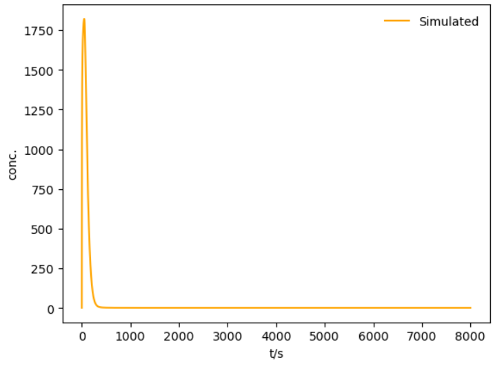
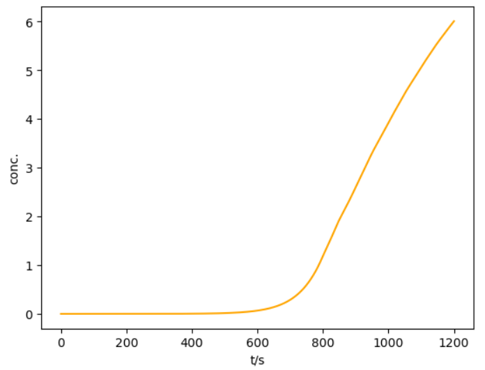
model = create_model(61.9, 473.8, 8.283e-12)
model.filename = 'model.h5'
model.save()
data = model.run()
model.load()
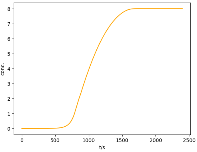
time = model.root.output.solution.solution_times
c = model.root.output.solution.unit_001.solution_outlet_comp_000 ## 1 mol/m^3 * 150 kg/mol=150 kg/m^3 = 150 mg/mL
fig = plt.figure()
ax = fig.add_subplot()
ax.plot(time, c*150, c="orange", label="Simulated")
ax.set_xlabel(r't/s')
ax.set_ylabel(r'conc.')
plt.show()
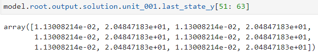
init_s = model.root.output.last_state_y
init_sdot = model.root.output.last_state_ydot
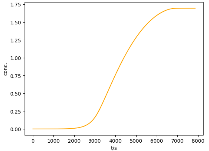
#### part II simulation
def create_model2(qmax, keq, Dp):
model = Cadet()
model.root.input.model.nunits = 3
model.root.input.model.unit_000.unit_type = 'INLET'
model.root.input.model.unit_000.ncomp = 1
model.root.input.model.unit_000.inlet_type = 'PIECEWISE_CUBIC_POLY'
model.root.input.model.unit_001.unit_type = 'GENERAL_RATE_MODEL'
model.root.input.model.unit_001.ncomp = 1
## Geometry
model.root.input.model.unit_001.col_length = column_length # m
model.root.input.model.unit_001.cross_section_area = column_volume/column_length # m^2
model.root.input.model.unit_001.col_porosity = column_porosity # 1
model.root.input.model.unit_001.par_porosity = particle_porosity # 1
model.root.input.model.unit_001.par_radius = 0.045e-3 # m
## Transport
model.root.input.model.unit_001.col_dispersion = 2.061e-8 # m^2/s
model.root.input.model.unit_001.film_diffusion = [1.18e-5] # m/s
model.root.input.model.unit_001.par_diffusion = [Dp,] # m^2/s
model.root.input.model.unit_001.par_surfdiffusion = n_sites * [0.0, ]
model.root.input.model.unit_001.adsorption_model = 'MULTI_COMPONENT_LANGMUIR'
model.root.input.model.unit_001.adsorption.is_kinetic = 0
model.root.input.model.unit_001.adsorption.mcl_ka = protein_MW*(1.0-total_porosity) * keq ## m^3 solid phase / mol protein / s ml/mg=m^3/kg 1 kda = 1 kg/mol
model.root.input.model.unit_001.adsorption.mcl_kd = kd ## s^-1
model.root.input.model.unit_001.adsorption.mcl_qmax = qmax/protein_MW/(1.0-total_porosity) ## mol/m^3 solid phase mg/ml=kg/m^3 / 150 kg/mol = 1/150 mol/m^3
model.root.input.model.init_state_y = init_s
model.root.input.model.init_state_ydot = init_sdot
### Grid cells
model.root.input.model.unit_001.discretization.ncol = 50
model.root.input.model.unit_001.discretization.npar = 12
### Bound states
model.root.input.model.unit_001.discretization.nbound = [n_sites]
### Other options
model.root.input.model.unit_001.discretization.par_disc_type = 'EQUIDISTANT_PAR'
model.root.input.model.unit_001.discretization.use_analytic_jacobian = 1
model.root.input.model.unit_001.discretization.reconstruction = 'WENO'
model.root.input.model.unit_001.discretization.gs_type = 1
model.root.input.model.unit_001.discretization.max_krylov = 0
model.root.input.model.unit_001.discretization.max_restarts = 10
model.root.input.model.unit_001.discretization.schur_safety = 1.0e-8
model.root.input.model.unit_001.discretization.weno.boundary_model = 0
model.root.input.model.unit_001.discretization.weno.weno_eps = 1e-10
model.root.input.model.unit_001.discretization.weno.weno_order = 2
model.root.input.model.unit_002.unit_type = 'OUTLET'
model.root.input.model.unit_002.ncomp = 1
model.root.input.solver.sections.nsec = 1
model.root.input.solver.sections.section_times = [0, 1.0*simulation_end_time1+1] # s
model.root.input.solver.sections.section_continuity = [0,0]
model.root.input.model.unit_000.sec_000.const_coeff = [c_feed] # mol / m^3; mg/ml = kg/m^3; 1 kda = 1 kg/mol 1.25/150
model.root.input.model.unit_000.sec_000.lin_coeff = [0.0]
model.root.input.model.unit_000.sec_000.quad_coeff = [0.0]
model.root.input.model.unit_000.sec_000.cube_coeff = [0.0]
model.root.input.model.connections.nswitches = 1
model.root.input.model.connections.switch_000.section = 0
model.root.input.model.connections.switch_000.connections = [
0, 1, -1, -1, Q,
1, 2, -1, -1, Q]
model.root.input.model.solver.gs_type = 1
model.root.input.model.solver.max_krylov = 0
model.root.input.model.solver.max_restarts = 10
model.root.input.model.solver.schur_safety = 1e-8
# Number of cores for parallel simulation
model.root.input.solver.nthreads = 1
# Tolerances for the time integrator
model.root.input.solver.time_integrator.abstol = 1e-6
model.root.input.solver.time_integrator.algtol = 1e-10
model.root.input.solver.time_integrator.reltol = 1e-6
model.root.input.solver.time_integrator.init_step_size = 1e-6
model.root.input.solver.time_integrator.max_steps = 1000000
# Return data
model.root.input['return'].split_components_data = 1
model.root.input['return'].split_ports_data = 0
model.root.input['return'].unit_000.write_solution_outlet = 1
# Copy settings to the other unit operations
model.root.input['return'].unit_001 = model.root.input['return'].unit_000
model.root.input['return'].unit_002 = model.root.input['return'].unit_000
# Solution times
model.root.input.solver.user_solution_times = np.linspace(0, 1.0*simulation_end_time1+1, simulation_end_time1+1)
return model
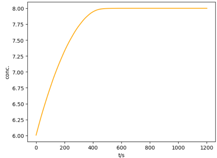
model = create_model2(61.9, 473.8, 8.283e-12)
model.filename = 'practice1.h5'
model.save()
data = model.run()
model.load()
time = model.root.output.solution.solution_times
c = model.root.output.solution.unit_001.solution_outlet_comp_000
fig = plt.figure()
ax = fig.add_subplot()
ax.plot(time, c*150, c="orange", label="Simulated")
ax.set_xlabel(r't/s')
ax.set_ylabel(r'conc.')
plt.show()