There are two approaches that I have followed over the course of my research. The one you should use depends on if you are employing single component or multicomponent models. The most important task is to convert UV into protein concentration, as you mentioned. You can also use the outlet conductivity and pH signals in the model if you apply the appropriate considerations, but this is usually optional.
Case 1) Single component
You can create a calibration curve to convert from UV to protein concentration: see Kumar et al. 2021 in JChromA and Altern et al. 2023 in JChromA (I followed the approach that @vijesh developed). The way this works is you prepare a series of protein samples at a wide range of concentrations by performing careful dilutions of a protein load sample above the highest concentration you expect to see in the outlet profile. I like to use a sample that is at least 10 mg/ml, but I primarily work with multimodal resins where the outlet protein concentration isn’t too high. The number of dilutions is entirely up to you, but more is better, especially if you use a wide range of concentrations. Be sure to use a calibration curve on your spectrophotometer (I use NanoDrop) to account for nonlinearity in the response. If you are using ion exchange resins under high loadings or affinity resins and performing step elution, the concentration go very high. In this case, you may need to concentrate your protein sample to reach an adequate concentration. The idea is that you don’t have to extrapolate here.
Next, you perform a series of injections using the diluted samples into the system in bypass mode. The samples should be at least 2 ml, depending if you use a sample loop or sample pump and how much dead volume you have in your system. You will know if it is enough sample when the resulting peaks reach plateaus and look like mini-breakthrough curves. Don’t forget to autozero after every injection, or make sure you treat peak height as the delta from each pre-peak baseline (often it is not zero). Once you are done, you fit the sample concentration against the UV peak height delta using a second order polynomial; i.e., C = aA^2 + bA, where a and b are fitting constants, A is the absorbance, and C is concentration. There should not be a c term constant because concentration should be zero at zero absorbance.
The reason why a second order polynomial is employed instead of a linear fit is because the response signal is very often nonlinear in ranges we like to use. In the case of UV 280 nm, the signal develops subtle nonlinear beyond 1500 mAU (from my experience) which becomes extreme near 3000 mAU, with complete saturation at around 3500 mAU. Depending on the path length of your flow cell and the concentration range of your experiment, you must choose a suitable wavelength. For example, UV 280 nm on a 2 mm flow cell will complete saturation at 15 mg/ml. UV 295 nm can be recorded at the same time to handle higher concentrations. The wavelength really matters and is important that you choose it correctly.
Once the calibration curve is prepared, you export the UNICORN data to an excel sheet and convert the UV signal to concentration. Beyond this, you just need to consider if there are any baseline shifts present and correct them if necessary.
A simpler approach for this entire experiment would be to use fewer samples and apply an apparent extinction coefficient. This will only work if the signal response is linear throughout all your experiments. Theoretically, you could choose a wavelength where this is the case, but clearly this approach is intrinsically limiting.
Case 2) Multicomponent
Case 1 assumes that your sample is pure or relatively pure. If this is not the case, the most straightforward approach is to collect fractions and analyze them offline. In my experiments I collect many fractions so I can have accurate data (either 0.5 CV or 1 CV fractions). You then analyze the samples for their concentration (I use nanodrop) and with an analytical assay to determine the composition. This ends up being a lot of work so there are a few ways to do this and different instruments to use. I found this method to be very consistent and also allows you to calculate the injection mass for the analytical assay which ensures your measurements are within the linear detection range (clearly the main takeaway of this post). Plate readers are more efficient than nanodrop but they are less accurate, in my opinion, so I always avoided them when running my own experiments. One reason why I don’t like it is because the applied path length is adjusted base on the fluid height, which is concentration dependent because of surface tension. The detection at low concentration is also more unreliable. So you get inaccurate data at both low and high concentrations. Another approach is to integrate the signals in your analytical assays to determine the concentration (based on a calibration curve). This can definitely work, but with this approach you cannot simultaneously determine both the concentration and composition accurately.
The approach that you follow depends on how accurate you need to be. Personally, I always try to have my experiments as accurate as possible because then if the predictions aren’t good, I can have confidence that the model is the issue and not my experiment.
Here are some examples of case 1) and case 2)
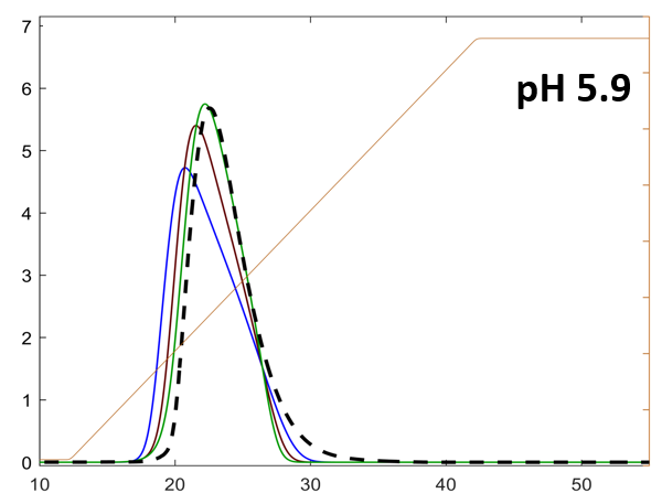
Case 1)
The axes are concentration [mg/ml] vs volume [ml]. The three lines correspond to predictions with different sets of isotherm parameters. The dotted black line is the experimental protein concentration.
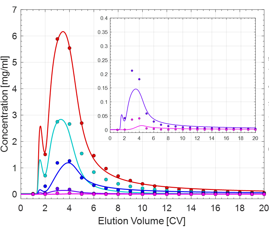
Case 2)
The different colored lines correspond to the individual protein components. The data points were determined via nanodrop followed by SEC and cIEF.
Hope this helps!
EDIT: don’t forget to account for dead volume in your post-processing if you don’t account tubing in your CADET model!