I want to create a CADET model that has a heterogeneous column porosity.
For that I build a test model that recreates a normal column by slicing it into several smaller columns. Each of the smaller columns have a slightly different column porosity. The total length as well as other parameters stay the same as a column with homogeneous column porosity.
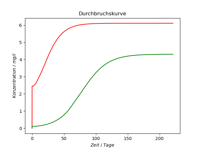
In theory my test model and a normal column should produce the same results if the column porosity is the same in each of the sliced columns in my test model.
Unfortunately that is not the case and I don´t know if I missed something.
Has somebody an Idea what the problem might be?
I just had a quick look into your code and could replicate your problem. We expect some minor differences as the discretization is not the same, however this should not be large when the discretization is fine enough. So I set the discretization higher and results did not change significantly, i.e. this does not explain the differences. Next, I reduced the problem gradually and found that the differences disappear, when particle reactions are neglected. I don’t know why that is, the model seems to be set correctly and the same for each column. I’ll think about it, maybe someone else has an idea in the meanwhile.
If you axially slice the column, the results will usually differ for two reasons, both of which are related to boundary conditions:
The higher order WENO reconstruction scheme is replaced by lower order methods towards the column boundaries. Hence, additional boundaries between shorter subsections will degrade the numerical performance, i.e. increase the approximation error for the same total number of volume elements. You can test this by using the first order upwind scheme instead of WENO.
Even using the upwind scheme, the results will still differ when the model accounts for column dispersion. This is because Danckwerts boundary conditions do not capture the dispersive flux in the downstream direction at the additional boundaries. You can test it by setting the dispersion coefficient to zero.
Note that you will need a very large number of axial volume elements to achieve a good approximation using the upwind scheme for problems without dispersion.
Thanks for the explanation Eric, please correct me if I misunderstood it.
Since I am not considering column dispersion in my model, the problem is mainly in the increased usage of lower order methods. That is because with the slicing of the column I create more boundary conditions for a column of the same size.
A way to minimize this problem would be the increase the axial discretization in order to decrease the relevance for the lower order methods for boundaries. (–> increase n_col)
Your other test option would be to change unit.discretization.weno.weno_order from 3 to 1.
Yes, exactly. With sufficiently many elements all numerical schemes should approximate the same test solution (with additional boundaries and same porosity).
Note that you will need a very large number of axial volume elements to achieve a good approximation using the upwind scheme for problems without dispersion.
What do you consider a very large number of axial volume elements?
n_col >100?
n_col >1000?
This is a good case to perform a brief screening of discretization granularity (i.e., try a bunch of simulations with different numbers of nodes). This way you can find the number of nodes that is suitable for your problem. You can do these simulations in parallel as well to perform it in a timely manner.
It is also important to remember that the number of axial nodes is relative to the length of the column in question—if you increase column length, you must increase the number of nodes to maintain consistency. I have found that when using the higher order WENO scheme that 24 nodes per cm of column is appropriate (beyond this point, there were no noticeable changes in results) for many types of simulations I have performed (working for both LRM and GRM). During parameter estimation, to decrease the workload, I have reduced this number to as low as 6 nodes per cm of column. In doing so, there were slight increases in peak broadness—presumably stemming from increased numerical dispersion. My point is that you can use reduced numbers of nodes, but should expect some changes in accuracy.
In the file you provided, the column length is set to 2.1 m; using the 24 nodes / cm “rule” would require 5,040 axial nodes, which is a lot—but this column is particularly long so it is to be expected. On top of this, if you need to increase the number of nodes due to the lower order scheme, the required number may be even higher.
In any case, I strongly recommend performing the aforementioned discretization screening which can be done using a basic grid search with simulations performed in parallel for efficiency. You can employ a residual calculation based on the difference between the simulation result with the test model and the result from the normal model, such that the minimum number of nodes can be found that still satisfies an appropriate error tolerance. If you want to get fancy with this and really save time, you can treat this as an optimization problem and solve it with a surrogate model which will really speed things up. I use surrogateopt in MATLAB (yes, I still use CADET-MATLAB) for all optimization problems and it is extremely useful. I have much less experience with Python, but one example I found is this package: Welcome to the pySOT documentation! — pySOT documentation
Does that mean that the porosity as a function of position is smooth / slowly varying?
Does it have jumps (e.g., do you expect to have zones in the column)?
The idea is to create a linear gradient along the whole column.
For example: the column is sliced into 4 sections first has a col_porosity of 0.45, the one after 0.43 the one after that 0.41 and so on.
Ideally the gradient between columns as well as the number of sliced columns (discretization of this col_porosity gradient) should be higher than my example.
I tried the setup with n_col=10000 and the weno order of 1.
Sadly there is no improvement. With a running time of 14 hours, any further increase in n_col is not really feasible.
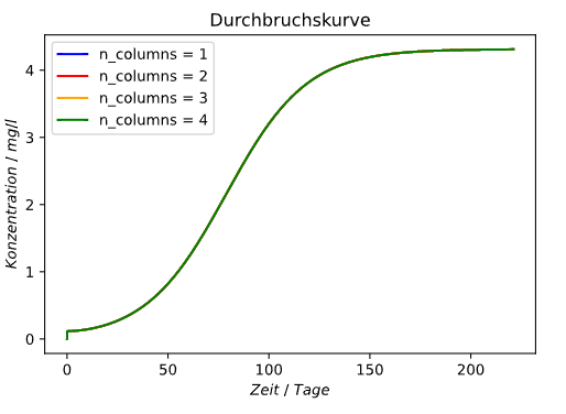
I found the issue.
We’ve been plotting the outlet of unit_001 instead of the outlet of the respective last column. The following code shows the expected behaviour for multiple columns: